the Creative Commons Attribution 4.0 License.
the Creative Commons Attribution 4.0 License.
 | 22 Mar 2018
Modeling of quasi-static thrust load of wind turbines based on 1 s SCADA data
Nymfa Noppe
Wout Weijtjens
Christof Devriendt
A reliable load history is crucial for a fatigue assessment of wind turbines. However, installing strain sensors on every wind turbine is not economically feasible. In this paper, a technique is proposed to reconstruct the thrust load history of a wind turbine based on high-frequency Supervisory Control and Data Acquisition (SCADA) data. Strain measurements recorded during a short period of time are used to train a neural network. The selection of appropriate input parameters is performed based on Pearson correlation and mutual information. Once the training is done, the model can be used to predict the thrust load based on SCADA data only. The technique is validated on two different datasets, one consisting of simulation data (using the software FAST v8, created by Jonkman and Jonkman, 2016) obtained in a controllable environment and one consisting of measurements taken at an offshore wind turbine. In general, the relative error between simulated or measured and predicted thrust load barely exceeds 15 % during normal operation.
- Article
(997 KB) - Full-text XML
- BibTeX
- EndNote


As the older wind farms slowly reach their designed lifetime, topics concerning fatigue, remaining useful lifetime and a possible lifetime extension gain importance. Moreover, as fatigue is a design driver for current offshore wind farms, fatigue analysis of existing wind turbines can optimize future design. Currently, fatigue assessments of support structures are often based on measurements of the load history (Iliopoulos et al., 2017; Loraux and Brühwiler, 2016; Schedat et al., 2016; Ziegler et al., 2017). Most of them imply continuous strain measurements at accessible locations. However, for several reasons accelerometers are preferred over strain gauges, although they are not suited to measuring quasi-static loads. In the research presented by Iliopoulos et al. (2017), the strain gauges are thus crucial to capture the quasi-static part of the loading. The research presented in this paper aims to replace the use of strain gauges for the estimation of quasi-static loads. Existing approaches to estimate thrust loads are based on simulations and additional design information (e.g., thrust coefficient) or acceleration measurements (Baudisch, 2012; Cosack, 2010).
Although supervisory control and data acquisition (SCADA) data are available for every wind turbine by default, their possibilities for load monitoring are still underutilized. Several authors (Hofemann et al., 2010; Vera-Tudela and Kühn, 2017) have suggested using 10 min SCADA statistics to estimate the loads on the blades. If the estimated model uses solely SCADA data, it can be translated to every turbine in the farm without the need of installing additional sensors. Recently, the use of 1 s SCADA signals has also become common practice in the industry. Therefore, the authors of this contribution propose to use 1 s SCADA data to estimate the thrust load, acting on the wind turbine and its substructure.
Although the authors will solely focus on the estimation of the thrust load, additional loads with higher frequencies contribute to fatigue as well. These additional loads are the result of rotor harmonics (3 p, 6 p, 9 p and in case of a rotor imbalance 1 p) and structural dynamics (first and second mode, FA1 and FA2). Figure 1a shows the frequency spectrum of measured bending moments, which illustrate the presence of the harmonics as well as the structural modes at an operational wind turbine. In the case of offshore wind turbines, an additional load is induced by waves. These additional wave loads cannot be coupled one on one with any SCADA parameter in time frames of a couple of seconds. Wind turbines installed on monopiles are more affected by waves than those installed on jacket substructures. An approach using SCADA data and accelerometers is proposed by Noppe et al. (2016) to account for the higher-frequency loads as well. However, it was concluded an improvement of the quasi-static model was needed. An alternative approach consists in using a reduced finite element model of the wind turbine and its substructure (Hartmann and Meinicke, 2017). Here, acting thrust loads are estimated using wind estimator software, which is not publicly available.
As explained, the thrust load has an important contribution to fatigue. However, it is also possible to associate the thrust with properties of wake flows. Therefore, an accurate estimation of thrust has also proved important in estimating wake wind speeds and turbulence (Réthoré, 2006).
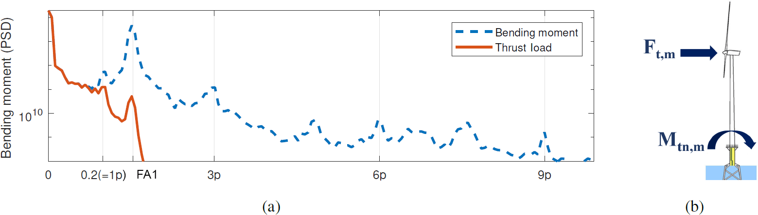
Figure 1(a) Frequency spectrum of measured tower bending moment in the fore–aft direction during 10 min (blue dashed line). The quasi-static part of the bending moment is filtered out (red solid line). The targeted quasi-static load (filtered) no longer contains the effects of rotor harmonics. (b) The measured thrust load Ft,m is obtained using the bending moment Mtn,m measured by strain gauges located at the interface between tower and transition piece.
2.1 Monitoring setup
To validate the proposed technique, results are shown using measurements taken at an offshore wind turbine. The monitored turbine is installed on a jacket and instrumented with strain gauges at the interface between transition piece and tower (Fig. 1b). The measured strains are converted into bending moments in the fore–aft and side–side directions using the turbine yaw in the SCADA. The quasi-static contribution of the thrust load to the measured bending moment Mtn,m is obtained by using a Butterworth filter of the fourth order on the recorded bending moments in a frequency range from 0 to 0.2 Hz. This frequency band is defined in a way so that the filtered signal is not influenced by the first natural frequency (0.31 Hz) since this is unrelated to any SCADA signal anyway. This is shown by the red solid line in Fig. 1a. The targeted quasi-static load (filtered) no longer contains the effects of structural dynamics and rotor harmonics.
The resulting signal is then transformed into thrust load Ft,m, using the distance between the sensors (location of the measured bending moment) and the hub (location of acting force) (Réthoré, 2006). To match the time steps of the SCADA data, the obtained thrust load is down-sampled using an antialiasing filter to a time frame of 1 s and additionally averaged over 10 min.
As the turbine is installed on a jacket, the role of wave loading in the bending moment is assumed to be negligible.
2.2 SCADA data
Every wind turbine is installed with a SCADA system. The main purpose of the SCADA system is to monitor and control plants, for which reason it records continuously. The main advantage of using SCADA data is the default availability. However, the correct calibration and quality of the sensors is not guaranteed over the entire lifetime. A common example is the anemometer to measure wind speeds and wind directions. It is installed behind the rotor and known for its high uncertainties due to poor calibrations. Moreover, the quality and accuracy of the data can differ among the different manufacturers. A proper preprocessing of the SCADA data and associated filtering process is advised. In this case, the preprocessing and filtering process consisted in exclusion of improbable and unrealistic values for wind speed (outside interval [0; 50] ms−1) and for generated power (outside interval [−0.1; 1.25] ⋅Prated) and periods of constant wind speed from the dataset. In total, less than 0.2 % is removed.
For this research a subset of 1 year of both 10 min statistics and 1 s signals of SCADA data was available. The subset consisted in both cases of measurements for wind speed, rotor speed, generated power, blade pitch angle, yaw angle and ambient temperature. Figure 2a shows the power curve obtained with 1 s and 10 min SCADA, respectively in blue and purple. The lines indicate the median value of the dataset, while the surface spans from the 5th to the 95th percentile of the data. The power curve shows a much higher variability for 1 s SCADA then for 10 min SCADA. The same difference in variability can be observed in Fig. 2b and c, where 1 s and 10 min averages of measured thrust load are plotted versus the 1 s and 10 min SCADA parameters wind speed and generated power, respectively. The present variability in 1 s data is not only the result of noise but is mainly due to the inertias within the controlling system and the wind turbine. For example, when the wind speed increases, the power output increases only a few seconds after. These inertias result in time delays of up to several seconds between, for example, the wind speed and the generated power. These delays are not considered constant over time and will differ for every SCADA parameter. Moreover, they last for only a couple of seconds and in consequence they cannot be observed within 10 min averages.
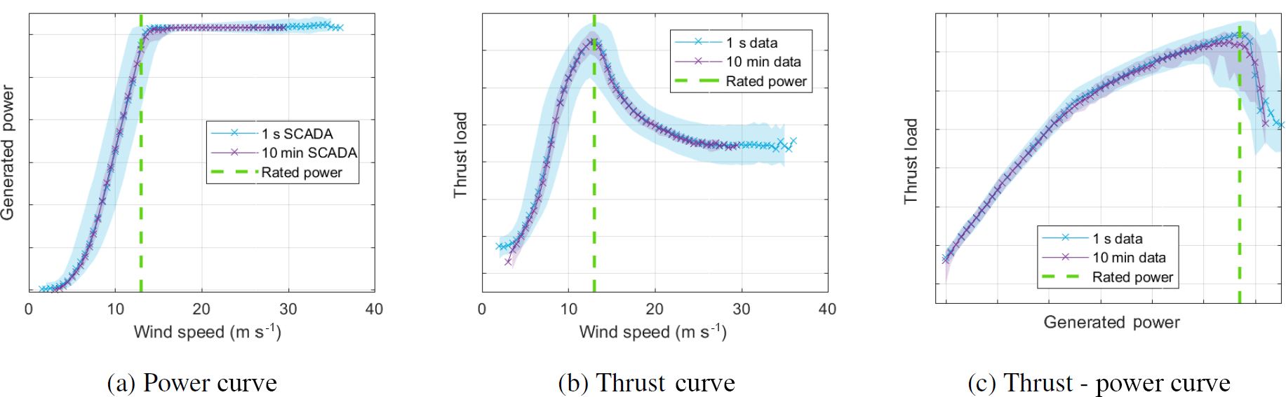
Figure 2Characteristic curves obtained using SCADA data in combination with averages of thrust load measurements. Operational data for a period of 2.5 months are shown. Data in both the 10 min time frame (blue) and 1 s time frame (purple) are shown. The line indicates the median value, calculated per bin of 0.5 ms−1 or 100 kW, whereas the surface spans from the 5th to the 95th percentile of the data. Rated power is reached for wind speeds of approximately 13 ms−1 (indicated by the green dashed line).
2.3 Meteorological data
Measurements of air pressure are available from a nearby met mast (15 km). Using the ambient temperature (from the SCADA dataset), the air density ρ is calculated using Eq. (1), where p is air pressure (Pa), T is ambient temperature (K) and Rspecific is the specific gas constant for dry air (287.058 ).
3.1 SCADA data
A crucial part in the model creation is the parameter selection. Input parameters are chosen based on their Pearson correlation and mutual information to the thrust load. The Pearson correlation between a thrust signal and all considered SCADA signals is calculated using Eq. (2), in which is the mean value of the signal X (May et al., 2011).
Since the problem we are facing is not necessarily linear, an analysis to identity and quantify possible chaotic or nonlinear dependence is recommended as well. A possible measure is mutual information, a measure of dependence based on information theory and the notion of entropy. The mutual information I(X;Y) between two signals X and Y is determined with Eq. (3) (Bonnlander and Weigend, 1994), using the probability density functions f(x), g(y) and h(x,y). To obtain these probability density function estimations, a histogram-based estimation as explained by Benoudjit et al. (2004) with bin widths defined using the interquartile range of the data, as suggested by Freedman and Diaconis (1981), is implemented. Opposed to Pearson correlation coefficients, mutual information does not have a general maximum value indicating perfect dependence between two signals. Therefore, the resulting mutual information should be normalized first. This is carried out by dividing by the joint entropy of the two signals (Bouma, 2009), as indicated by Eq. (3).
The calculation of Pearson correlation and mutual information is performed for operational data only, both 1 s data and 10 min data, for a period of 2.5 months. During this period the full wind speed range is covered, as shown by Fig. 2. Additionally, the datasets are divided into two subsets: data when the turbine was operating below rated operation (64 % of 10 min and 62 % of 1 s operational data) and at rated operation (36 % of 10 min and 38 % of 1 s operational data).
The resulting Pearson correlation and mutual information between the measured thrust load and several SCADA parameters for all datasets is depicted in Fig. 3.
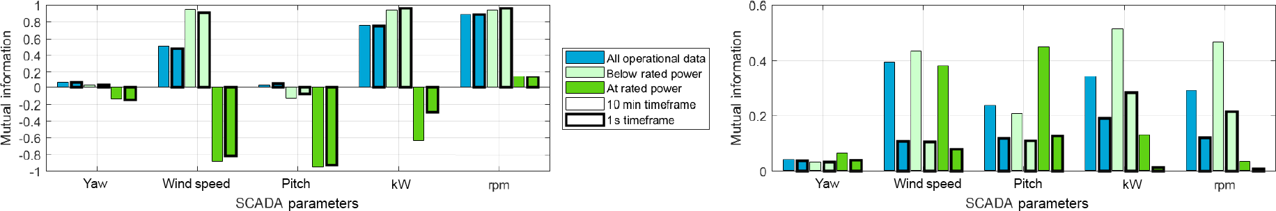
Figure 3The Pearson correlation is calculated between thrust load averages and five standard SCADA parameters for operational data only. Both 10 min and 1 s averages are considered. The total dataset is divided based on the operational state of the turbine (operating below rated power and operating at rated power).
Focusing first on the results for the total operational dataset, a high Pearson correlation can be found for rotor speed (0.8871 and 0.8935 for 10 min and 1 s data, respectively), generated power (0.7513 and 0.7497) and to a lesser extent wind speed (0.5082 and 0.4829). When looking at the results of mutual information for the total operational datasets, the highest dependencies are again found for wind speed (0.3934 and 0.1068 for 10 min and 1 s data, respectively), generated power (0.3453 and 0.1904) and rotor speed (0.2888 and 0.1217). Interestingly, a relatively high value is also found for the blade pitch angle (0.2330 and 0.1186). In the case of the operational data below rated power, the values for Pearson correlation and mutual information are even higher for rotor speed (0.9383 and 0.9622 for Pearson correlation and 0.4660 and 0.2161 for mutual information), generated power (0.9396, 0.9603, 0.5158 and 0.2811) and wind speed (0.9417, 0.9086, 0.4342 and 0.1057). Here, the values for mutual information of pitch angle decreased to 0.2075 and 0.1103 for the 10 min and 1 s datasets, respectively, since the pitch angle does not vary a lot as long as generated power is below rated. Conversely, operational data at rated power reveal a high Pearson correlation of the blade pitch angle (0.9499 and 0.9298) and wind speed (0.8898 and 0.8194). The same observation is made for the results of mutual information: 0.4492 and 0.1268 for the blade pitch angle and 0.3804 and 0.0793 for the wind speed. This difference in behavior is explained as follows. Once the turbine reaches its rated power value, the only parameter acting to vary wind speed and thrust load will be the blade pitch angle. Hence a significantly lower correlation and mutual information for the rotor speed (0.1562, 0.1385, 0.0333 and 0.0098) is found. However generated power is still correlated to thrust load with a significant value in the case of 10 min averages (0.6354). The value for mutual information in the case of 10 min data is significantly higher as well (0.1308). Figure 2c reveals a very steep curve between thrust and generated power once rated power is reached.
In the results of Pearson correlation (Fig. 3, left) negative values are the result of an additive inverse relationship between the depicted parameter and the thrust load. For a turbine operating below rated power, a higher wind speed results in a slightly lower blade pitch angle and an increased thrust load. Therefore, a decreasing blade pitch angle (due to an increase in wind speed) leads to a higher thrust load. Hence, a negative value for Pearson correlation between pitch angle and thrust load when the turbine is operating below rated power is expected. Once rated power is reached, increasing wind speeds result in higher blade pitch angles, slightly increasing generated power and decreasing thrust loads (Fig. 2b). Accordingly, an increase in blade pitch angle and generated power (thanks to an increase in wind speed) enforces a decrease in thrust load. And thus, a resulting negative Pearson correlation between thrust load and wind speed and generated power and pitch angle for operational data at rated power is consistent.
It is obvious the turbine reacts differently to varying wind speeds depending on the operational state. Once rated power is reached, the relation of the thrust load to the depicted SCADA parameters often differs. This leads to lower correlation values for the total dataset in comparison to the operational states separately. In the case of the pitch angle, the correlation is even nonexistent when looking at the total operational dataset. However, when taking into account the existing nonlinearities, as with mutual information, the blade pitch angle is clearly correlated with the thrust load based on the total operational dataset as well.
In general the values for Pearson correlations and clearly for mutual information are less considering 1 s averages compared to 10 min averages. This can be explained by the present time delays of several seconds between parameters, as a result of the inertias present within the system. When calculating the autocorrelation between the thrust load signal and shifted SCADA signals, the biggest time shift was found for the pitch signal and corresponded to −3 s.
For the continuation of this research, only the yaw angle will not be considered as an input parameter due to its small correlation and mutual information (0.0598, 0.0596, 0.0403 and 0.0367 for Pearson correlation of 10 min and 1 s datasets and mutual information of both datasets, respectively) with the thrust load.
3.2 Meteorological data
According to Baudisch (2012), thrust loads are influenced by air density. While changes in the depicted SCADA variables happen within seconds, air density changes on a different timescale (several hours). Instead of including air density in the set of input parameters, it is accounted for as a correction of the modeled thrust load : .
Seeing that the relation between thrust load and the depicted SCADA parameters is nonlinear, a model will be created using a neural network. A neural network is capable of finding and characterizing nonlinear dependencies within datasets. Therefore, it can handle the inverted relations between thrust load and the considered SCADA parameters once rated power is reached. The neural network used in this paper has three hidden layers with four neurons each. By choosing a different topology the root-mean-square error of the test set improved with a maximum of 0.2 % if more than one neuron was chosen in each layer.
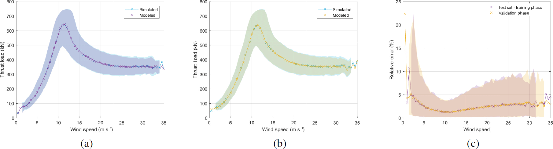
Figure 4Modeled and simulated thrust loads for the total dataset during the training phase (training, validation and test set combined, simulated time of 2.5 days) (a) and the total dataset during the validation phase (1.5 days) (b). The relative error (c) for the test dataset during the training phase and the additional dataset during the validation phase (simulated time of 1.5 days) is shown as well. The lines indicate median values for every wind speed bin of 0.5 ms−1; the surface spans from the 5th to the 95th percentile of the data.
It is trained using operational data only, while operating both below and at rated power. The training data consisted of 1 s SCADA data and 1 s averages of thrust load measurements (FT,m_training). The input parameters chosen are wind speed, blade pitch angle, rotor speed and generated power, as concluded in Sect. 3. To account for the inertias in the system, not only instantaneous SCADA values but also the values of five previous seconds are included in the model. Since the model will be used in every normal operational state of the wind turbine, it is important that the full operational wind speed band is covered in the training dataset. For every operational state, e.g., during a down-rating or curtailment, that is not represented in the training data, the model will probably not be able to predict the thrust load correctly.
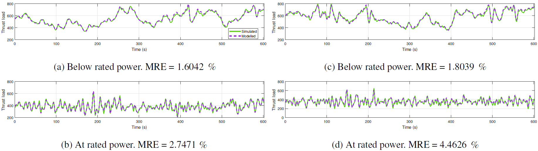
Figure 5Time series (spanning 10 min) of modeled and simulated thrust loads below rated (a, c) and at rated power (b, d). For each operational state, the time series with the highest averaged absolute error is shown (c, d). MRE shows the averaged absolute relative error over 10 min.

Figure 6Modeled and measured thrust loads for the training data (training, validation and test set combined, being 2 weeks worth of data) (a) and the long-term validation data (1 year worth of data) (b). The relative error (c) for the test dataset during the training phase and the dataset of 1 year during the validation phase is shown as well. The median values for relative errors obtained with the test set of FAST simulations are copied.
To train the neural network, the Neural Network toolbox of MATLAB is used with the default settings (Guide, 2002). This means the preprocessing is performed with a min–max mapping function, tan-sigmoid transfer functions are used for hidden layers and a linear transfer function is used for the output layer. Furthermore, the data chosen to train the model are randomly divided into 70 % training data, 15 % validation data and 15 % test data. This so-called hold-out method is preferred over cross-validation to reduce the computational load since large datasets are used. Training is carried out using the training data and the Levenberg–Marquardt algorithm. Training of the network is stopped when the error on the validation data failed to decrease for six iterations or a maximum number of 1000 iterations is reached. The test data are used as an independent dataset of the network training to calculate the final model error.
As explained in Sect. 3.2, the effect of air density is accounted for by applying a correction on the model results. To make sure the effect of air density is not present in the training data, the inverse correction is applied on the measured thrust loads of the training dataset: .
The modeling method proposed in Sect. 4 is validated using two different datasets. The first one is obtained by simulation in FAST, while the second one is obtained thanks to a measurement campaign performed at an offshore wind turbine. The dataset obtained using simulations was included to illustrate the approach in a controlled and reproducible environment.

Figure 7Time series (spanning 10 min) of modeled and measured thrust loads below rated (a, c) and at rated power (b, d). For each operational state, the time series with the highest averaged absolute error is shown (c, d). MRE shows the averaged absolute relative error over 10 min.
5.1 FAST simulations
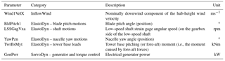
The simulated data are obtained by using the software FAST v8 (Jonkman and Jonkman, 2016), offered by the National Renewable Energy Laboratory (NREL). The chosen simulated turbine is the NREL 5.0 MW baseline wind turbine, installed on an OC3 Monopile RF configuration. All simulation specifications are kept as proposed by the software (Jonkman and Jonkman, 2016) for use of this turbine type. This means that turbulence and irregular waves are also accounted for. To make sure the full wind speed range is sufficiently covered in the simulation data, several input wind files with varying average wind speed between 3 and 25 ms−1 are generated using TurbSim. Each wind speed is accounted for equally. In essence, the wind distribution is thus considered uniform.
The output parameters of interest for this research are specified in Table 1. As the results obtained using simulated data will be used to be compared to real-life data, only comparable parameters for the SCADA data and the measured bending moment are worked with and indicated in Table 1.
The air density is kept constant during the simulations. Therefore, the applied corrections for air density did not influence the results.
To train the model, a dataset with a total simulated time of ca. 2.5 days is used. Additionally, the model is validated on an additional simulated dataset with a total simulated time of ca. 1.5 days. These data are not used to train the model and can thus be used as a complete independent validation set.
Results are shown in Fig. 4. A good match between modeled thrust load and simulated thrust load FT,s can be found during both training and validation phases (Fig. 4a, b). Figure 4c shows the relative error Δϵ between simulated and modeled thrust load () versus wind speed for the test set during the training phase and the total dataset during the validation phase. The line indicates the median value of the relative error, calculated for each wind speed bin of 0.5 ms−1. The surface spans from the 5th to the 95th percentile of the data. In general, the relative error of both datasets barely exceeds 10 %, except for very low wind speeds. Here, a higher relative error is found due to the lower absolute values of the thrust load. For higher wind speeds, errors increase. Starting from 12 ms−1 an increasing variability in relative error can be observed for increasing wind speed. A similar behavior was found for the training and the validation set during the training phase. This indicates the training set was representative for the validation set, the test set and the total dataset during the validation phase.
Four time series spanning 10 min during the validation phase are shown in Fig. 5, two while operating below rated power (Fig. 5a, c) and two while operating at rated power (Fig. 5b, d). The time series of 10 min with the highest averaged absolute error between simulated and modeled thrust loads below rated and at rated power are shown in Fig. 5c and d, respectively. In all cases a very good match is found. This is represented by a low value for the averaged absolute relative error (MRE) for those time series (MRE > 4,5 %).
5.2 Application to real world: offshore wind turbine
The proposed modeling method is also tested on an operating wind turbine. Thrust loads are measured using strain gauges, installed at the interface between tower and transition piece, as explained in Sect. 2. A model is trained using 2 weeks of 1 s data. Moreover, this model is validated on a dataset of 1 year, including the 2 weeks of training data.
Results are shown in Fig. 6. A good match between measured thrust loads FT,m and modeled thrust loads can be found during both training and validation phases. Although above roughly 18 ms−1, the modeled thrust curve shows less variability than the measured curve, meaning the difference between the 5th and the 95th percentile of modeled thrust is lower than the difference between the 5th and the 95th percentile of measured thrust (Fig. 6a, b). Figure 6c shows the relative error () of the test set during the training phase, being 15 % of the total training set of 2 weeks, and the total dataset during the validation phase of 1 year of operation. Again, the line indicates the median value, calculated for every wind speed bin of 0.5 ms−1. The surface spans from the 5th percentile to the 95th percentile of the data. A similar behavior among the training, validation and test set during the training phase was obtained. In general, the relative error does not exceed 15 %. Moreover, with a median value barely exceeding 5 %, results are promising. In general, the errors are increased with respect to the results using FAST (as shown in Fig. 6c). The errors obtained for lower wind speeds up to 10 ms−1 are increased due to offsets, the mean differences between measured and modeled values, present in the results. When looking at the long-term validation set, the errors are increased with respect to the test set during the training phase due to bigger mean differences. Furthermore, the errors obtained for wind speeds higher than ca. 18 ms−1 are slightly higher due to the loss of variability in the tail of the thrust curve. Again, an increasing variability in relative errors can be observed for increasing wind speeds, starting from ca. 12 ms−1.
To illustrate these observations, four time series of 10 min are shown in Fig. 7. Two of them show operation below rated power (a and c), while the other two show operation at rated power (b and d). The time series depicted in Fig. 7c and Fig. 7d show 10 min with the highest averaged absolute error when operating below or at rated power, respectively. An offset can be observed in (a, c), while the loss of variability can be observed in (d). The values of the averaged absolute relative error indicate the match is still acceptable (MRE < 6.5 %). As explained, the resulting errors are influenced a lot by present offsets between the measured and the modeled thrust load signal. However, these offsets will not influence a fatigue assessment performed according to common practice in industry. This practice consists of cycle counting of the stress signals and transforming the cycle counts into damage using the Miner's rule. Since during this practice only the size of the cycles matters, the fatigue assessment is not influenced by the mean value of the cycles.
Calculating the Pearson correlation and the mutual information between the measured and modeled thrust load signals for the same period of 2.5 months (see Sect. 3) results in 0.9962 and 0.2740, respectively. These increased values for 1 s data signals indicate that a lot of the present variability in the thrust load can be explained by combining several SCADA parameters and allowing some latency between the different signals. When looking at only one parameter, the difference in value for thrust measurements occurring for the same value of that parameter cannot be explained. When considering more parameters, this difference might already be explained by a different value of another parameter. Therefore, the resulting correlation between the measured thrust load and only one parameter is lower than between the measured thrust load and a combination of multiple parameters, as performed by the neural network.
An approach to estimate thrust load signals based on SCADA signals is explained and validated both on simulation and real measurement data. Wind speed, rotor speed, blade pitch angle and generated power are selected as input parameters based on both a linear and a nonlinear correlation analysis. Strain sensors are used to measure the acting thrust load. This thrust load signal is combined with SCADA signals to train a neural network. Validation of the method is carried out using FAST simulation data and data measured at an offshore wind turbine during 1 year. Time series show a good match between modeled and measured or simulated thrust signals. In general, the relative error barely exceeds 15 %. Results obtained using FAST data are slightly better than those of the real-world offshore wind turbine.
Essential in this approach is the preprocessing of the SCADA data. Moreover, including an air density correction proved to reduce offsets in the results. Furthermore, good results are obtained even when using the default settings of the neural network toolbox in MATLAB. Adjusting the neural network hyperparameters, e.g., number of layers and neurons, did not improve the results significantly.
The use of 1 s SCADA data can be considered as the main advantage of this approach. If the model proves to be transferable among turbines of the same type, this approach can be applied on any (non-instrumented) wind turbine within a wind farm. This transferability should be validated using cross-validation among instrumented turbines.
The method presented is capable of estimating quasi-static loads on wind turbines. To perform a full fatigue assessment of wind turbines, structural and rotor dynamics have to be accounted for as well. For offshore wind turbines with significant wave loading, e.g., large diameter monopiles, the effect of waves on the structure also needs to be included. A full load reconstruction can be performed by combining the proposed approach with acceleration measurements (Noppe et al., 2016).
Seeing that the data are proprietary to the industrial partner of this project, the data used in this paper cannot be made publicly available.
The authors declare that they have no conflict of interest.
This work has been funded by the Institute for the Promotion of Innovation by
Science and Technology in Flanders (IWT) in the framework of the VIS OWOME
Project and by the Research Foundation – Flanders.
Edited by: Gerard J. W. van Bussel
Reviewed by: two anonymous referees
Baudisch, R.: Structural health monitoring of offshore wind turbines, Ph.D. thesis, Master's thesis, Danmarks Tekniske Universitet, 2012. a, b
Benoudjit, N., François, D., Meurens, M., and Verleysen, M.: Spectrophotometric variable selection by mutual information, Chemometr. Intell. Lab., 74, 243–251, http://citeseerx.ist.psu.edu/viewdoc/download?doi=10.1.1.28.576&rep=rep1&type=pdf, 2004. a
Bonnlander, B. V. and Weigend, A. S.: Selecting input variables using mutual information and nonparametric density estimation, in: Proceedings of the 1994 International Symposium on Artificial Neural Networks (ISANN'94), 42–50, 1994. a
Bouma, G.: Normalized (pointwise) mutual information in collocation extraction, Proceedings of GSCL, 31–40, 2009. a
Cosack, N.: Fatigue load monitoring with standard wind turbine signals, Ph.D. thesis, Universität Stuttgart, Stuttgart, 66–75, 2010. a
Freedman, D. and Diaconis, P.: On the maximum deviation between the histogram and the underlying density, Probab. Theory Rel., 58, 139–167, 1981. a
Guide, M. U.: Neural network toolbox, The MathWorks, Chapter 2, http://www.image.ece.ntua.gr/courses_static/nn/matlab/nnet.pdf, last access: July 2002. a
Hartmann, S. and Meinicke, A.: Model based lifetime estimation of support structures using Kalman Filter, presentation at GIGAWINDlife Symposium, 2017. a
Hofemann, C., van Bussel, G., and Veldkamp, H.: Forecasting of wind turbine loads based on SCADA data, 6th PhD Seminar Wind Energy, p. 17, 2010. a
Iliopoulos, A., Weijtjens, W., Van Hemelrijck, D., and Devriendt, C.: Fatigue assessment of offshore wind turbines on monopile foundations using multi-band modal expansion, Wind Energy, 20, 1463–1479, 2017. a, b
Jonkman, J. and Jonkman, B.: NWTC information portal (FAST v8), https://nwtc.nrel.gov/FAST8, last access: 27 July 2016. a, b
Loraux, C. and Brühwiler, E.: The use of long term monitoring data for the extension of the service duration of existing wind turbine support structures, J. Phys. Conf. Ser., 753, 072023, https://doi.org/10.1088/1742-6596/753/7/072023, 2016. a
May, R., Dandy, G., and Maier, H.: Review of input variable selection methods for artificial neural networks, in: Artificial neural networks-methodological advances and biomedical applications, edited by: Suzuki, K., InTech, 19–44, 2011. a
Noppe, N., Iliopoulos, A., Weijtjens, W., and Devriendt, C.: Full load estimation of an offshore wind turbine based on SCADA and accelerometer data, J. Phys. Conf. Ser., 753, 072025, https://doi.org/10.1088/1742-6596/753/7/072025, 2016. a, b
Réthoré, P.-E.: Thrust and wake of a wind turbine: Relationship and measurements, Technical University of Denmark (DTU), 32–44, 2006. a, b
Schedat, M., Faber, T., and Sivanesan, A.: Structural health monitoring concept to predict the remaining lifetime of the wind turbine structure, in: Domestic Use of Energy (DUE), 2016 International Conference on the IEEE, 1–5, 2016. a
Vera-Tudela, L. and Kühn, M.: Analysing wind turbine fatigue load prediction: The impact of wind farm flow conditions, Renew. Energ., 107, 352–360, 2017. a
Ziegler, L., Smolka, U., Cosack, N., and Muskulus, M.: Brief communication: Structural monitoring for lifetime extension of offshore wind monopiles: can strain measurements at one level tell us everything?, Wind Energ. Sci., 2, 469–476, https://doi.org/10.5194/wes-2-469-2017, 2017. a