2.1 Turbine simulation

Throughout this paper, we use FAST, NREL's aeroelastic simulation tool (Jonkman, 2013). FAST is a widely used industry and academic tool for wind turbine load estimation. NREL's WISDEM software allows for the execution of FAST and its companion tool TurbSim (which generates turbulent wind fields for input to FAST) in a programmatic fashion from Python, as has been reported previously (Graf et al., 2016).

The particular turbine on which we are testing these methods is the NREL 5 MW reference turbine, often used for such studies (Choe et al., 2016; Jonkman et al., 2015), in an onshore configuration. The environmental conditions are thus described by hub height mean wind speed (modeled by a Weibull distribution with scale and shape parameters of 11.28 m s⁻¹ and 2, respectively). Additional environmental parameters of turbulence intensity, spectrum, coherence function, and wind shear are kept fixed at nominal values. It should be noted that the stochasticity in the combined TurbSim–FAST simulation comes from the random seed that is input to TurbSim. This seed governs the exact starting conditions for the generation of the turbulent inflow wind field. Because this is an ergodic system, a long enough simulation would eventually cover all possible wind conditions. However, for finite simulations, multiple runs using different random seeds allow us to sample the space of all possible turbulent flow field snapshots with the same mean wind speed, turbulence intensity, etc. This is common practice in extreme load analysis. We can regard random seed as a proxy for sampling over a uniform distribution of turbulent inflows for each set of environmental conditions.

For this study, we selected two output channels of interest, tower base side–side bending (“TwrBsMxt” in FAST nomenclature) and tower base fore–aft bending (“TwrBsMyt”), which provide contrast because the wind speeds at which their highest loads occur overlap differently with the typical wind speed distribution. The side–side moments grow with hub height wind speed, making their extremes hard to estimate with traditional MC sampling because they do not overlap well with typical wind distributions. The fore–aft counterparts do overlap quite closely with the typical wind distributions.

2.2 Extrapolation

The current standard for estimating extreme loads relies on extrapolation. We refer the reader to the relevant literature for a detailed exposition of the extrapolation method (Graf et al., 2017; Moriarty, 2008; Ragan and Manuel, 2008; Toft et al., 2011). Here we present a concise statement of the method and discuss one or two subtleties. The protocol to construct exceedance curves using binning and extrapolation is as follows:

1. Run TurbSim–FAST N_i times per wind speed x_i at the center of bin i (typically N_i∼6).

2. For each bin i, concatenate the data from each seed and extract peaks (see below regarding peak extraction and timescales). For future reference we refer to the resulting dataset as {Y_i,k}, where i indexes over wind speed bins and k indexes over the peaks we have extracted at that wind speed.

3. For each bin i, form empirical cumulative distribution functions (CDFs) and fit a chosen distribution $F_i\left(x\right)=P(Y<l|x)$ to them. In this paper we use a three-parameter Weibull distribution.

4. (Optional). For each bin, convert each fitted distribution to the desired timescale (see below regarding peak extraction and timescales).

5. Finally, $P(Y<l)=$ $\int P(Y<l|x\left)f\right(x)\mathrm{d}x$ $\sim {\sum }_{i}P(Y<l|x_i\left)f\right(x_i)\mathrm{\Delta }{x}_i$, where f(x) is the probability density function (pdf) of wind distribution, and Δx_i is the width of bin i. The probability of exceedance is the complementary distribution $P(Y>l)=\mathrm{1}-P(Y<l)$, and its estimate is $\widehat{P}(Y>l)=\mathrm{1}-{\sum }_{i}P(Y<l|x_i\left)f\right(x_i)\mathrm{\Delta }{x}_i$.

The distributions chosen to fit the bin-wise CDFs are the theoretically appropriate extreme value distributions (generalized extreme value (GEV), three-parameter Weibull, etc.). However, this does not mean they accurately represent the behavior of the particular FAST loads in a specific context. The optimality properties of extreme value distributions are asymptotic properties, but we are performing “intermediate asymptotics”: long-term – but not infinitely long-term – trends. Nevertheless, these distributions are the appropriate starting point.

In this paper we are using a three-parameter Weibull distribution, but this is not meant as a claim that this choice is better than any other in the literature (Gumbel, GEV, etc). We used the three-parameter Weibull because we have used it with success in previous work (Graf et al., 2017). There are many excellent studies examining the choice of distribution and the method of extracting peaks (Dimitrov, 2016; Moriarty, 2008; Naess and Gaidai, 2009; Ragan and Manuel, 2008; Toft et al., 2011), but this is not the focus of the present work.

Regarding the fitting procedure, in light of the interest in extrapolation, rather than just fitting, we have fit the empirical CDF of the data directly to the theoretical CDF of the distribution by nonlinear least squares. We have done this separately for the data from each wind speed bin. Furthermore, in order to emphasize the largest peaks (i.e., the lowest probability values) we do not use all the data, just the M_pks largest peaks in each bin, where M_pks is an algorithmic parameter. M_pks plays a role in our studies similar to the threshold used in peak-over-threshold methods, but for purposes of connecting to the bin-based approach it has the advantage that there are always the same number of peaks extracted from a given length simulation. As an exercise, we experimented with using different values of M_pks, as discussed below in Sect. 4 and illustrated in Fig. 2. The broad conclusion is that there is a window of values of this parameter that provides similar performance, which suggests this parameter will not be an impediment to practical implementation of this algorithm.

It is important to be clear regarding various time spans at play here. First, there is the ultimate time of interest, typically in wind studies the 50-year return period. This does not mean that in 50 years the event in question happens with a probability of 1. Sometimes it is loosely defined as an event having a probability of 1∕50 of happening in 1 year. Strictly speaking it is an event that happens on average one or more times in 50 years according to a Poisson process whose events-per-interval parameter is one in 50 years. Next there is the simulation time, i.e., the length of each FAST run. This is almost always 10 min in the literature. In relation, there is the time span over which our estimates of exceedance probability apply. These are also traditionally 10 min, i.e., reported probabilities of exceedance are probabilities of exceedance in 10 min, but there is nothing in principle to make this fixed. Finally, there is the length of time between independent peaks. This time can be estimated empirically by examining the autocorrelation of the data; values as low as 4 s have been justified in previous studies (Ragan and Manuel, 2008), and 10 s seems to be more than adequate.

The various time spans come into play as we extract peaks and make estimates. The rule that connects them is the simple AND rule of probability: if Y<l for time T, and T=Kt, then Y<l for time t for K times in a row, so $P_T(Y<l)=P_t(Y<l{)}^K$. For probabilities of exceedance P(Y>l), we write $P(Y>l)=\mathrm{1}-P(Y<l)$ and use the same idea, resulting in the familiar expression $P_T(Y>l)=\mathrm{1}-(\mathrm{1}-P_t(Y>l){)}^K$. For example, the former is typically used to convert peak distributions collected on a 10 s, 1 min, or peak-over-threshold basis to a 10 min basis, while the latter is used when we derive the ubiquitous value of 3.8 × 10⁻⁷ that represents the probability of the 50-year return period event happening in 10 min.

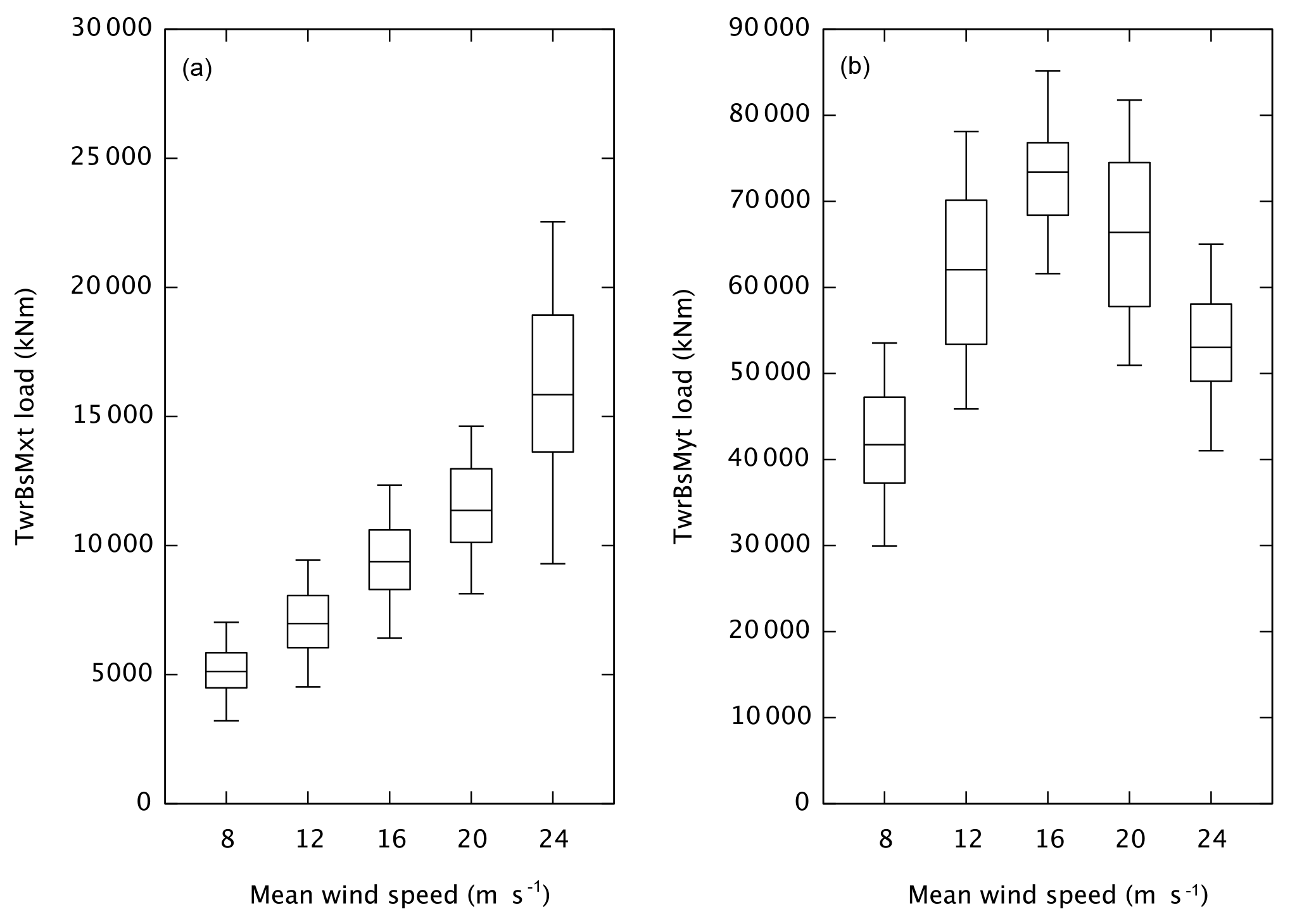
Figure 1Box-and-whisker plots of the distribution of the raw response (specifically, all 1 min maxima) of the combined TurbSim–FAST simulation as a function of wind speed bin for side–side (a) and fore–aft (b) loads. The difference in general trend between side–side and fore–aft loads is clearly evident. The variability within each bin is extreme (especially for the fore–aft load), which puts an upper bound on the utility of sampling methods (e.g., IS) targeting certain wind speeds. The boxes show the median and 25th and 75th percentiles. The whiskers are positioned at the 5th and 95th percentiles. The data are the absolute maxima in 1 min segments of 120 separate 10 min simulations per bin (1200 total peaks for each bin).

Download

In this paper we adopt the following setup: all our simulations are 11 min long, for which we discard the first minute as a transient and retain the final 10 min for our studies (we will occasionally be loose with the terminology and refer to these as “10 min simulations”). To gather peaks, we take the maximum of each 1 min segment in our simulations. This provides exactly 10 peaks per simulation, which allows for building 1 min empirical CDFs (i.e., probability of exceedance in 1 min) in a consistent manner. The resulting 1 min empirical POEs are converted to 10 min POEs as described above (i.e., K=10) to conform to standard practice. Below we experiment with how many of these peaks should be used in the fitting of the extreme value distributions used in the extrapolation method. This alternative to the peak-over-threshold method makes comparison and correspondence between extrapolation and sampling easier, because we have a fixed number of peaks per FAST run. The tradeoff between gathering more peaks (at the risk of sacrificing statistical independence) versus fewer peaks (at the risk of not having enough data) is an algorithmic detail that we could study further, but it is not the focus of this paper. Our motivation for using 1 min interval peak separations is to pick a reasonable point along this tradeoff that avoids the pitfalls of either extreme. Finally, we have divided the wind speed range into five bins centered at 8, 12, 16, 20, and 24 m s⁻¹.

To acquire a sense of the basic variability in the response, we have run 20 independent sequences of the simulations described above for the extrapolation method (six random seeds per bin). Figure 1 consists of box-and-whisker plots of the peaks from the first 6000 peaks (10 peaks per run × 6 seeds × 20 repetitions × 5 bins). For both the side–side and fore–aft loads, the variability within each bin is large. For example, the difference between the 95th and 5th quantiles for the 24 m s⁻¹ side–side bin is comparable to its median value. For the side–side load the dependence on wind speed is clearly also very strong, whereas for the fore–aft load, the variability within the bins is as large as it is between the bins. A detailed study of response variability in the context of offshore wind turbine fatigue loads is given in Zwick and Muskulus (2014).

2.3 Monte Carlo importance sampling for extreme loads

MC methods are widely used to estimate expectations of quantities calculated using stochastic simulations (Robert and Casella, 2004). IS is an MC method in which an auxiliary importance distribution q(x) is used to focus sampling on areas of the target distribution f(x) that are most relevant with respect to the functions of interest (e.g., the loads Y(x)). Often relevant means minimal variance (see below). The broad applicability of the method arises from the so-called IS identity:

where E_f and E_q represent the expectation with respect to f and q, respectively. This means, from an MC standpoint, that both

and

(where M_tot is the total number of samples we have of the quantity we are estimating) are unbiased estimates of the same quantity E_f[Y(x)].

For us M_tot will be the number of peaks gathered from the FAST runs. In what follows we will use M to represent numbers of peaks and N to represent numbers of FAST runs. With our convention of taking the maximum over 1 min spans of 10 min simulations, we will have M=10N throughout. The subscript “tot” will be the total number (over all bins), whereas index subscripts (e.g., “i”) will refer to the peaks or runs within the corresponding bin. Thus as above, N_i is the number of FAST runs (i.e., random seeds) in the ith bin, M_i=10N_i is the number of peaks extracted from the N_i runs, and N_tot is the total number of FAST runs.

Although the estimates above in Eqs. (5) and (6) are both unbiased, they could have drastically different variance, which means that they may converge at drastically different rates. The minimal variance importance distribution can be derived and is

From a practical standpoint there are two obvious problems with this result. First, it depends on the expectation we wanted to calculate in the first place. This objection we can overcome using some form of accept–reject sampling that does not depend on the normalization constant. (As long as we can evaluate Y(x), even if by simulation (we assume we can also evaluate f(x)), we can sample from any distribution proportional to Y(x)f(x) using the accept–reject algorithm (see, e.g., Robert and Casella, 2004), which involves sampling uniformly in a 2-D region containing the function Y(x)f(x). The probability of x with respect to the Y×f distribution is just the proportion of these uniform samples below Y⋅f in this 2-D box. This procedure does require assumptions on the bounds of Y and the support of Y and f, but in principle these can be made large enough to sample any reasonable probability Y⋅f). A more significant problem, however, is that q^* also depends on the function Y(x) whose expectation we are trying to calculate with as few evaluations as possible. Finally, in our case, an even worse problem is that Y(x) is not a deterministic function of x; thus, as stated, q^* is also a stochastic function. Nevertheless, Eq. (7) provides a guide for our quest to find the minimal variance importance distribution: it should be as close as possible to proportional to the product of load Y(x) and wind probability f(x).

For our purposes, finally, note that Eq. (1) can be written as an expectation of the so-called “indicator” function that is 1 if Y(x)>l and 0 otherwise:

Equations (1) and (8) form the basis of the mathematical bridge between extrapolation and the MC–IS methods described in Sect. 3.

2.4 IFORM

The following section is not essential to understanding our adaptive IS algorithm and may be considered optional. However, we believe it provides useful conceptual context, especially to understand the limits of statistical methods for systems whose response variability is large. Here, keeping in mind the goal – minimal variance unbiased estimates of extreme loads through IS, minimizing the use of extrapolation – we summarize the IFORM and EC methods. IFORM was introduced by Winterstein (Winterstein et al., 1993) and addresses the estimation of extreme loads from a different perspective. Instead of directly computing the integral in Eq. (1), IFORM seeks to find the combined set of environmental conditions and resulting loads that have a desired joint return period probability. The EC variant explicitly separates the environment from the turbine's response to it, in effect being a method that seeks to directly find the conditions that cause the extreme load.

In the general IFORM approach, the combined environmental and response variable space is considered to be one joint probability distribution, and the quantile corresponding to the desired return period is explored to find the maximal response. In practice, the distribution of the environmental part of this combined space is assumed known. For example, in this paper, the environmental component is wind speed, which is assumed to have a Weibull distribution with a shape and scale of 11.28 m s⁻¹ and 2, respectively. Then response data are gathered for samples in the environmental space, and a conditional distribution “response given the environment” is fit to these data, which allows finally for extrapolation to the desired return period. This use case of IFORM is thus a form of extrapolation, with its strengths (it requires very few samples to build arbitrarily low POE estimates) and weaknesses (there is no guarantee, as outlined above, that extrapolation outside the range of data, i.e., from short to long times, is valid). In this sense everything we can say about using adaptive IS to reduce the variance of traditional extrapolations applies to IFORM estimates as well. The more data we have in the relevant bins, the more accurate our statistical fits and resulting extrapolations will be.

The EC variant of IFORM explicitly separates environment from response. It works best if the response of interest is a completely deterministic function of environmental conditions that themselves have known probability. Then one can directly search the environmental contour (e.g., all wind–wave–turbulence combinations that occur on average once in 50 years) to find the highest load. Otherwise, a conditional distribution of response subject to environment can model the response variability away from its median; in this case, EC is then similar to IFORM in practice. Together, IFORM and EC solidify the important notion of response variability: the magnitude of the variation in the nonlinear stochastic response for fixed environmental conditions.

These notions help to explain why IFORM or EC applied to wind turbine extreme loads estimation may not be much different than other extrapolation methods. On the one hand, as noted above, though systematic and efficient, IFORM relies on extrapolation. Just like the standard extrapolation method, it relies on being able to extrapolate from easily observable quantiles (5th, 25th, 50th, 75th, 95th, etc.) to the very difficult to observe quantiles corresponding to the 50-year return period. On the other hand, EC is not applicable when the main driver of variation in a system is the response variability, which (see Fig. 1) is largely the case for wind turbines; the main driver of extreme loads is not a particular wind speed but some idiosyncratic chaotic process that even for a prosaic wind speed just might come together to cause an extreme load.

The present task, that of estimating extreme loads with wind speed as the only environmental variable, is governed mostly by the response variation. Therefore we will not estimate extreme loads by IFORM in this paper. However, IFORM is critical for conceptual understanding: where possible, our goal should be to convert response variation (intractable) to environmental variation (tractable) through better understanding of its physical cause. It is the extreme response variability (different random seeds for the same environmental conditions can cause very different FAST output because they cause very different turbulent inflow) that makes extreme load estimation a difficult problem. We return to this subject in Sect. 5.

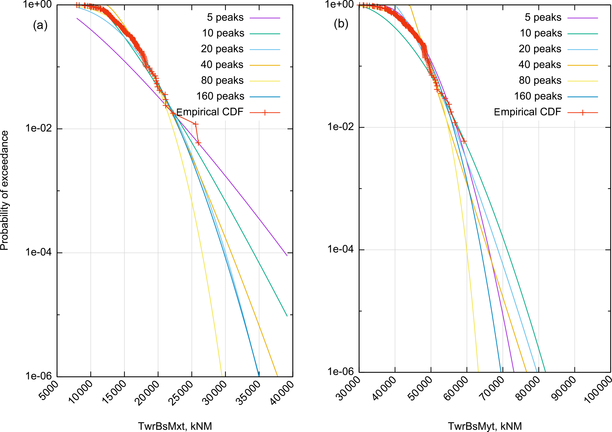
Figure 2Weibull three-parameter fits to the empirical CDF for the wind speed bin centered at 20 m s⁻¹ for a variety of choices for how many peaks M_pks we use for the fit for side–side (a) and fore–aft (b) tower base loads. In all cases we are fitting the analytical CDF to the highest M_pks loads of the empirical CDF (a lower value of M_pks is like a higher threshold in the peak-over-threshold method). Especially for the side–side moment, the extrapolated POE values depend heavily on how many peaks are used.

Download

3.1 Bin-wise empirical CDFs as the bridge between extrapolation and MC

When we perform the bin-wise simulations used in the extrapolation methods, we are performing stratified sampling. Recognizing that these samples can be described as a probability distribution provides a bridge to using them in an IS context, as discussed in Graf et al. (2017). The basic idea is as follows. Assume a set of samples {x_i} from an arbitrary distribution g(x) of wind speeds (g may be either f(x), q(x), or an empirical one derived from binning the data). By running FAST, the set {Y_i} of corresponding loads can be generated and sorted from the lowest to the highest. Then for any given load Y_j, the IS estimate is

Letting $w_i\equiv \frac{f\left(x_i\right)}{g\left(x_i\right)}$, we can concisely write the empirical CDF for all the loads {Y_j} as

To apply this formula to data from the binning method, we need the appropriate g(x), i.e., the appropriate weights w_i of each sample. Recall, we write the dataset as {Y_i,k}, where i indexes over wind speed bins and k indexes over peaks extracted at that wind speed. We rewrite the integral over wind speeds as a sum of integrals, and then approximate each separate integral by the M_i peaks derived from the N_i runs (in our case, over TurbSim random seeds) at the fixed wind speed x_i for bin i:

From this, we see that the “weight” contributed by sample i,k to the probability of non-exceedance (1-POE) of Y_j is $\frac{\mathrm{1}}{M_i}f\left(x_i\right)\mathrm{\Delta }{x}_i$ for all i,k such that $Y_{i,k}<Y_j$. To calculate the empirical CDF from the bin data, then, we assign weight $w_i=\frac{\mathrm{1}}{M_i}f\left(x_i\right)\mathrm{\Delta }{x}_i$ for all samples from bin i and apply Eq. (15). Table 1 summarizes the exact correspondence between extrapolation and IS–MC. The importance density corresponding to stratified sampling is seen to be

We note that g(x) is in fact normalized:

This is important because it ensures our importance weights $w_i=f\left(x_i\right)/g\left(x_i\right)$ are ratios of two normalized densities.

Table 1Bin-wise empirical cumulative distribution functions provide a bridge from extrapolation, which builds POE from bin-wise fitted distributions F_i, and importance sampling, which builds an unbiased estimate from the appropriately defined distribution g.

Download Print Version | Download XLSX

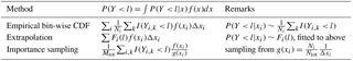
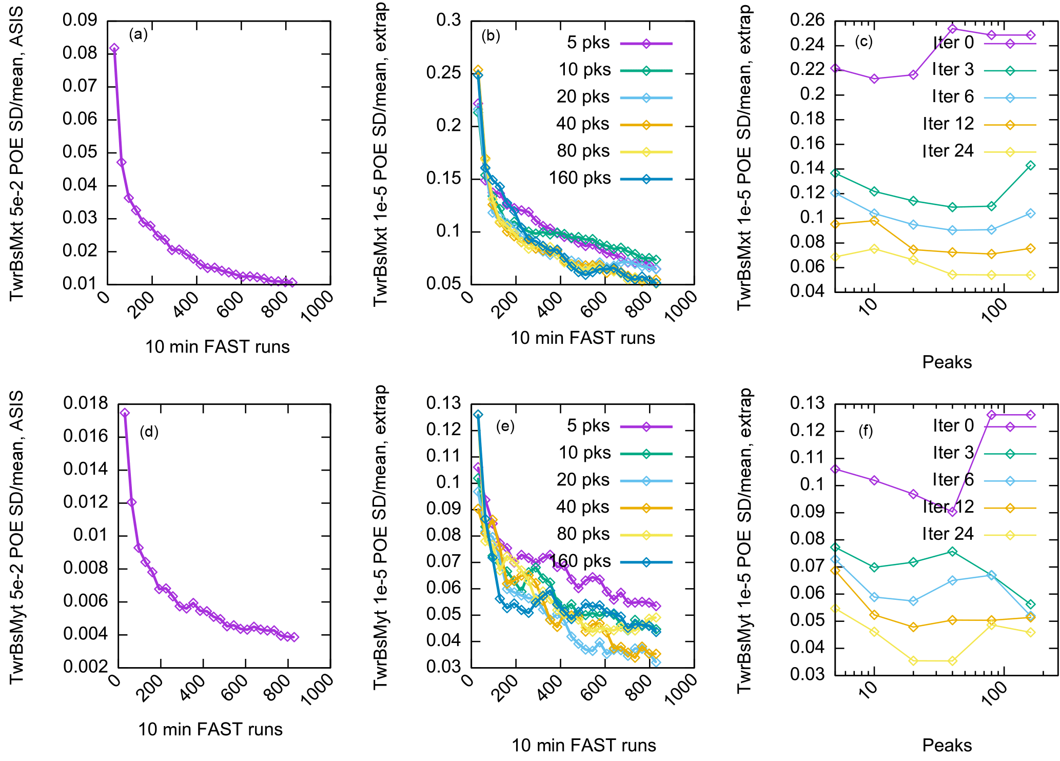
Figure 3Summarizing the convergence of tower base load estimates using extrapolation and ASIS estimates over 100 independent runs. The top row is side–side; the bottom is fore–aft. The y-axis units are the ratio of the standard deviation to the mean estimate (relative standard deviation, measuring convergence). The x axis is the number of FAST runs (measuring computational expense). The target POE for the empirical ASIS estimate (a, d) is 5 × 10⁻² and for the extrapolation estimate (b, c, e, f) is 10⁻⁵. Adaptively selecting samples, in a way designed to accelerate the convergence of the empirical estimate (ASIS, a, d), also accelerates the convergence of the extrapolation estimates (b, c, e, f). There is a somewhat weak dependence on the number of peaks used for extrapolation, but M_pks∼40 appears robust for both loads. The side–side load estimate has larger initial relative variance because (as shown above in Fig. 1) its extremes occur at high winds, but its relative variance is reduced more quickly by the adaptive procedure than the fore–aft load.

Download

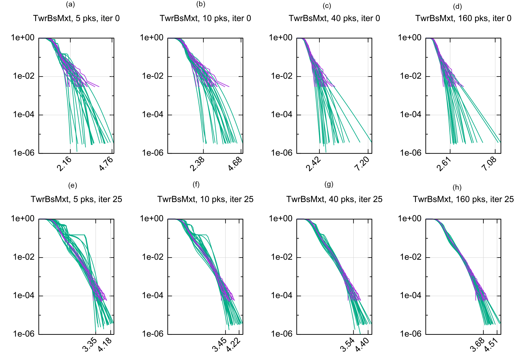
Figure 4Behavior of ASIS and iterative updating of extrapolation for side–side tower base bending load over 20 separate runs as a function of M_pks. The x-axis units are 10 000 s of kilogram newton meters; the y axis is probability of exceedance in 10 min. The top row shows the results of both ASIS and extrapolation at iteration 0 (i.e., just based on the initial set of bin-wise samples) as a function of the number of peaks used for fitting the extrapolation distributions. The bottom row shows the estimates after 25 ASIS iterations. (Note the ASIS results are the same across each row because they are independent of M_pks.) Clearly the variance of the estimates is tightened. It is not clear from visual inspection if one choice of M_pks is better than any other.

Download

Figure 5Behavior of ASIS and iterative updating of extrapolation for fore–aft tower base load over 20 separate runs. The x-axis units are 10 000 s of kilogram newton meters; the y axis is probability of exceedance in 10 min. The format is the same as Fig. 4. Again it is interesting to compare the visual representation with the statistics presented in Fig. 3. The single extremely large load discovered by ASIS was also seen in Graf et al. (2017) (f). Though it is beyond the scope of the present paper to do so, one of our main conclusions is that the statistical methods have come to a point at which the best course forward will be to pursue the exact causes of such loads and integrate a statistical description of such situations into our methods.

Download

Thus we have a “bridge” between fitting and sampling. Bin-wise empirical CDFs can be directly compared with fitted distributions (in fact, they are what we fit to). But the estimate over all wind speeds can then be expressed generically in the IS language suited to comparison with MC and IS estimates. IS–MC methods do not provide any bin-wise information (there are no bins); thus it is otherwise impossible to “debug” their divergence from extrapolation. This formulation allows us to see, first, that error accrues from lack of convergence of empirical CDFs, for both methods. Additionally though, for extrapolation, the error is compounded by lack of fit between the chosen extreme value distribution and the empirical CDFs, which is the price we pay for being able to extrapolate to arbitrarily low POEs with small numbers of samples.

3.2 ASIS as stochastic optimization

The discussion above indicates that the samples from the bin-based methods can alternatively be used to make empirical estimates via their implied importance distributions. This orientation suggests, also, that there is no barrier to changing the distribution of samples as we go. Thus we can think of the estimation procedure as an optimization problem: find the distribution of bins (number of samples per bin) that results in unbiased estimates with minimal variance. In Graf et al. (2017) we have used a heuristic algorithm that looked for “gaps” in the empirical peak distribution. Here instead we introduce a gradient-based approach. As above, let N_i be the number of FAST runs performed in the ith wind speed bin, and let N be the vector of bin counts. Now, the variance of the estimate using importance distribution g is

Note the second term does not depend on g (in the corresponding integral, the g in the denominator cancels out). Thus

Here we have used the fact that $\frac{M_i}{M_{\mathrm{tot}}}=\frac{N_i}{N_{\mathrm{tot}}}$ to write the expression in terms of bin counts instead of peak counts.

Our algorithm begins by running the standard six seeds per bin from the extrapolation method (i.e., N_i is initialized to 6 for all i). Then we perform the following steps in an iterative fashion.

1. Compute ∇_NJ(N).

2. Allocate a target number of new samples (e.g., 20 per iteration) to bins in two ways:

   • a.

     allocate some percentage of the new samples in proportion to ∇_NJ;

   • b.

     recognize this is a global optimization problem, and allocate the rest to other bins randomly.

3. Run TurbSim–FAST for the new batch.

4. Append the new peak data to the existing data and update our empirical estimates of POEs and our extrapolation estimates using the cumulative data according to Eqs. (15) and (18).

Note the algorithm as stated does not explicitly recognize the stochasticity of the underlying quantity Y(x). Because we are using an unbiased estimate of the gradient of the variance, our approach, naive as it is, is known to converge “almost surely” to a local optimum (Robbins and Monro, 1951). In fact it is a form of stochastic gradient descent (Goodfellow et al., 2016). Casting the problem in this form allows for taking advantage of ongoing research in this area. There are two reasons for step 2b of the algorithm. First, it is not clear a priori that our optimization problem is convex. Thus there could be multiple local minima. Step 2a and 2b correspond to the tradeoff between exploitation and exploration common to all global optimization algorithms. Second, because the gradient is calculated from an unconverged statistical estimate, there is an error associated with this vector. Preventing unconverged estimates from steering us in the wrong direction is an additional reason to include the exploration step 2b.

A slight complication comes from the need for the N_i to be integers (we can only have an integer number of runs per wind speed bin). Currently we simply round N_i to the nearest integer. Thus we are following the gradient as closely as possible subject to the integral nature of N_i. We claim that this is a reasonable procedure because the variance of the estimates is observed to be a rather slowly varying function of the bin distribution; thus taking the nearest feasible (i.e., integral N_i) point to the point suggested by our gradient will incur a bounded and likely small error. Also, the gradient itself is an estimate, not an exact value, so we are already working with inexact quantities from the standpoint of traditional gradient-based optimization. A more refined approach we could explore in the future is to apportion simulation time spent in each bin according to N_i. This would amount to a relaxation (from the discrete space to the continuous space Parker and Rardin, 1988) of the problem and would allow for exactly following the (albeit still stochastic) gradient.

Next, as stated J only concerns one load type (e.g., tower base side–side bending moment). But previously (Graf et al., 2017) and above (i.e., Fig. 1) we have seen that side–side and fore–aft loads favor different importance distributions. Since it defeats the purpose of the method to have to repeat it for every load, we have adopted an “umbrella” concept; we compute the desired bin distribution for all the loads of interest, and form the minimal superset of bins that includes them all. Also, note that the gradient (e.g., see Eq. 22) is always negative; increasing any bin count will reduce the variance, which makes obvious sense. The purpose of the algorithm is to guide the distribution of bin counts to have optimal proportions from each bin. Our current implementation works in a cumulative fashion. At every iteration, we are always adding more simulations, never removing them.

Another issue, even for a single load type, is how many of its peaks Y_i are considered in computing the gradient of the variance. We remind the reader that ASIS per se does not require any extrapolation. This question of how many peaks to use to compute ∇_NJ(N) is different from the question of how many peaks M_pks to use for extrapolation. It is another algorithmic parameter that one could tune. Using all the peaks would reduce the variance of the POE estimates of all the peaks, even the small peaks we do not care about. Using just the single largest peak would overemphasize the bin that this single peak happened to come from. The choice of the five largest peaks is rather arbitrary, enough so that more than the single largest peak contributes, but not so many as to deemphasize the goal of finding large peaks.

Finally, because we are still refining the mechanics of the algorithm, ASIS as stated does not include a stopping criteria. Since what ASIS minimizes is the variance of our load estimates, stopping should be based on driving the variance below a user-defined threshold. The difficulty, of course, is that unlike a deterministic gradient descent procedure, our only access to the actual variance is through further statistical estimates. In the results below we simply repeat the stochastic optimization procedure 100 times and compute the variance of the estimated loads directly. A less computationally expensive approach is bootstrapping (Fogle et al., 2008; Sultania and Manuel, 2017), which we would recommend for a production implementation of ASIS. In bootstrapping, the variance of our load estimates is estimated as follows: At every iteration, there are M_i peaks extracted from the N_i runs at wind speed x_i for bin i. Normally we use these directly in Eq. (15) to form a single POE estimate. Instead, in bootstrapping, we resample the M_i peaks with replacement some number, say L, of times to form L resampled sets of peaks, all of length M_i, but all containing different subsets of the original M_i peaks. These are used to compute L independent POE estimates, from which an empirical variance can be computed and used for stopping criteria.