2.1 Eddy lifetime

A number of forms exist to estimate eddy lifetime τ_e, though these can be generally expressed as the ratio of a length scale (taken as the reciprocal of wavenumber, k⁻¹) to a velocity scale which follows from some integrated form of the (scalar) kinetic energy spectrum E(k):

where the characteristic velocity scale can be generically described by

In contrast to the “coherence-destroying diffusion time” of Comte-Bellot and Corrsin (1971) and the reciprocal of eddy-damping rates from Lesieur (1990), for use with rapid-distortion theory Mann (1994) chose an eddy lifetime that depends on eddy size (wavenumber) according to

i.e., equivalent to p=0 in terms of Eq. (1). The choice of Eq. (2) for eddy lifetime was found to behave more reasonably than both the Comte-Bellot and Corrsin (1971) “diffusion time” (where p=1)², as well as the timescale $\left[k^{\mathrm{3}}E\right(k){]}^{-\mathrm{1}/\mathrm{2}}$ (which in the inertial range is equivalent to $p=-\mathrm{1}$)³ implicit in eddy-damped quasi-normal Markovian models (Andre and Lesieur, 1977; Lesieur, 1990); both of the latter lifetime models do not (reliably) integrate to give finite ${\mathit{\sigma }}_u^{\mathrm{2}}$.

Mann (1994) re-writes τ_M as

where ₂F₁ is Gauss' hypergeometric function (Abramowitz and Stegun, 1972)⁴, and L_MM is the turbulence length scale associated with the peak of the turbulent kinetic energy spectrum E(k) as in Eq. (2). The eddy lifetime definition (3) is used in practical implementation of the spectral tensor model (Mann, 2000), and it notably defines a parameter of this model: the eddy lifetime factor Γ, also known as the anisotropy factor. The Mann (1994) spectral-tensor model employs RDT, whereby the shear dU∕dz distorts turbulence from an isotropic state, based on an initial turbulent kinetic energy spectrum of the von Kármán form

where α=1.7 (von Kármán, 1948). This in effect defines the length scale L_MM through the peak of the initial spectrum⁵. Using Eq. (4) in the proportionality expression (2) produces

where we have introduced the proportionality constant c_τ to write the result of integrating the proportionality relation (2) as an equation. Now τ_M can be seen to depend upon k, L_MM, and ε. The eddy lifetime can be reduced and clarified via ${}_{\mathrm{2}}{F}_{\mathrm{1}}\left\{\frac{\mathrm{1}}{\mathrm{3}},\frac{\mathrm{17}}{\mathrm{6}};\frac{\mathrm{4}}{\mathrm{3}},(-k{L}_{\text{MM}}{)}^{-\mathrm{2}}\right\}\simeq [\mathrm{1}+\mathrm{3.07}(k{L}_{\text{MM}}{)}^{-\mathrm{2}}{]}^{-\mathrm{1}/\mathrm{3}}$ to give the more transparent von Kármán-like form⁶

Since Eqs. (3) and (5) are equal, we have an expression relating the Mann-model parameters to the shear dU∕dz:

The expression (7) can be made yet more useful to relate the turbulent length scale to measurable parameters, as shown in Sect. 2.2.

2.2 Characteristic length scale

Noting that the spectrum of a variable integrates to the variance of said variable, then invoking Eq. (8) with the isotropic von Kármán form Eq. (4) for E(k) and exploiting $F_{\mathrm{11}}\left(k_{\mathrm{1}}\right)=\int \int {\mathrm{\Phi }}_{\mathrm{11}}\mathrm{d}{k}_{\mathrm{2}}\mathrm{d}{k}_{\mathrm{3}}$, one obtains the isotropic streamwise turbulence variance

which is the undistorted streamwise variance. The factor 0.69 is the numerical value of $\frac{\mathrm{9}}{\mathrm{55}}\sqrt{\mathit{\pi }}{f}_{\mathrm{\Gamma }}\left(\frac{\mathrm{1}}{\mathrm{3}}\right)/f_{\mathrm{\Gamma }}\left(\frac{\mathrm{5}}{\mathrm{6}}\right)$, and f_Γ(x) is the Euler gamma function (Abramowitz and Stegun, 1972). Then using Eq. (9) in Eq. (7) we get a relation for the isotropic (undistorted) turbulence length scale implied by the lifetime model (3),

where the leading term in parentheses is expected to be of the order of 1.

2.3 Ideal neutral surface-layer implications

Within the atmospheric surface layer (ASL), in the homogeneous stationary limit under neutral conditions, $\mathrm{d}U/\mathrm{d}z\to u_{*}/\left(\mathit{\kappa }z\right)$ so that Eq. (11) reduces to $L_{\text{MM}}\to c_m\mathit{\kappa }z\approx \mathrm{0.92}z$. Similarly, in this “log-law regime” ${\mathit{\epsilon }}_{\text{ASL,N}}=u_{*}^{\mathrm{3}}/\left(\mathit{\kappa }z\right)$ so that Eq. (7) becomes ${\mathrm{\Gamma }}_{\text{ASL,N}}=c_{\mathit{\tau }}(\mathrm{3}\mathit{\alpha }/\mathrm{2}{)}^{-\mathrm{1}/\mathrm{2}}(L_{\text{MM}}/\mathit{\kappa }z{)}^{\mathrm{2}/\mathrm{3}}$, or equivalently $L_{\text{MM}}{|}_{\text{ASL,N}}=(\mathrm{3}\mathit{\alpha }/\mathrm{2}{)}^{\mathrm{3}/\mathrm{4}}\mathit{\kappa }z[\mathrm{\Gamma }/c_{\mathit{\tau }}{]}^{\mathrm{3}/\mathrm{2}}$, which via Eq. (12) can be written

Thus for $c_m={\mathit{\sigma }}_{\text{u,obs}}/u_{\text{*,obs}}$, we see that the Mann (1994) eddy-lifetime formulation (3) implies $L_{\text{MM}}\to \mathrm{1.1}\mathit{\kappa }z({\mathit{\sigma }}_{u,\text{obs}}/{\mathit{\sigma }}_{\text{iso}}{)}^{\mathrm{3}/\mathrm{2}}$ in the neutral ASL. Meanwhile, as noted just above, the mixing-length form (11) implies L_MM→c_mκz; this is consistent with Eq. (19) under the condition that $({\mathit{\sigma }}_{u,\text{obs}}/{\mathit{\sigma }}_{\text{iso}})\simeq (c_m/\mathrm{1.1}{)}^{\mathrm{2}/\mathrm{3}}$ or roughly ${\mathit{\sigma }}_{u,\text{obs}}\approx \mathrm{1.6}{\mathit{\sigma }}_{\text{iso}}$ for c_m≃2.3.

3.1 Testing of assumptions and predicted constraints

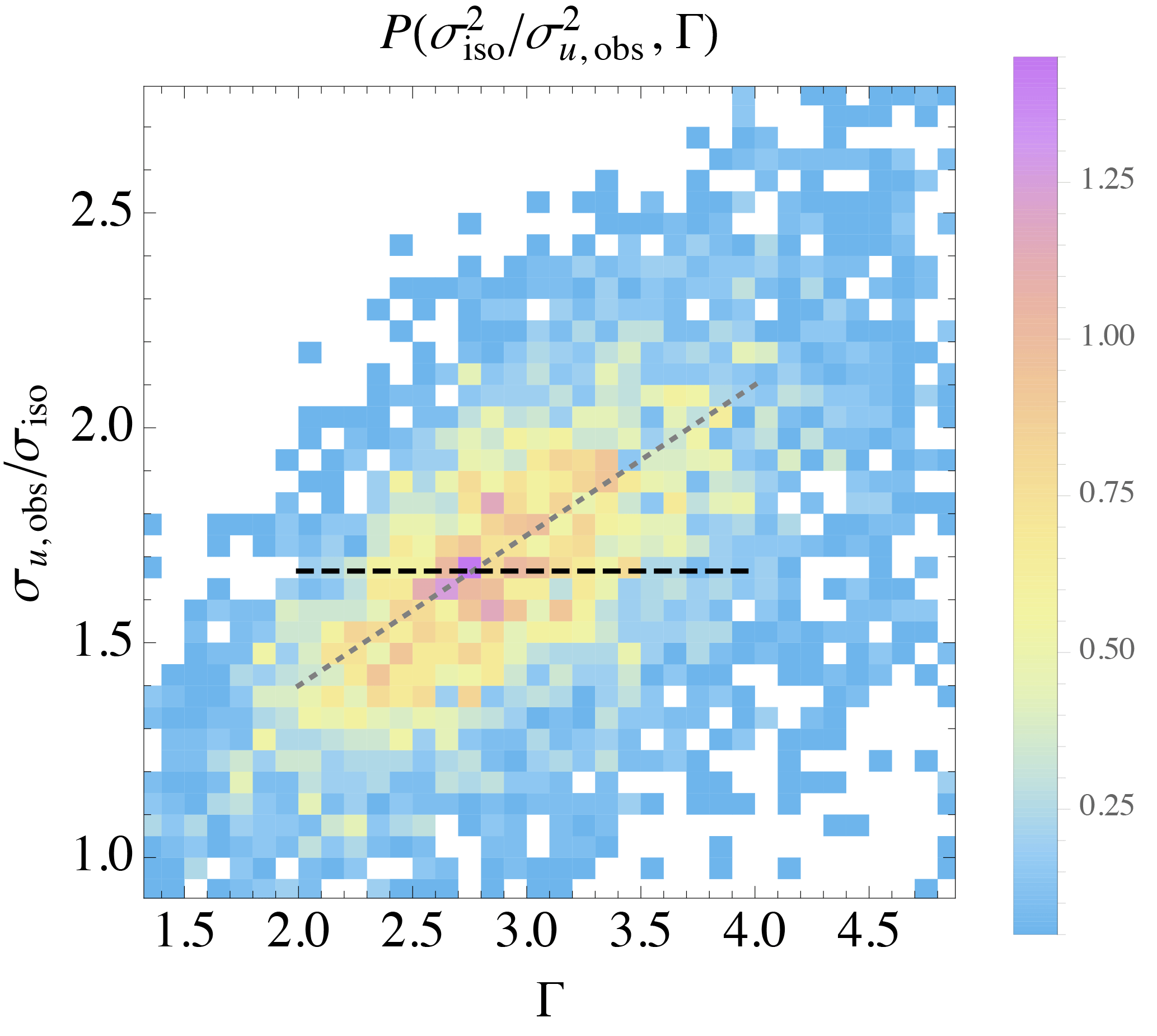
The implications of Eqs. (12)–(15) included the independence of L_MM and c_τ from Γ, as well as (for example) the expected dependence ${\mathit{\sigma }}_{u,\text{obs}}\propto \mathrm{\Gamma }{\mathit{\sigma }}_{\text{iso}}$. Indeed we find that L_MM is independent of Γ, with no significant statistical correlation: $\langle L_{\text{MM}}\mathrm{\Gamma }\rangle /\sqrt{\langle L_{\text{MM}}^{\mathrm{2}}\rangle \langle {\mathrm{\Gamma }}^{\mathrm{2}}\rangle }<\mathrm{0.15}$ for land or sea sectors at any given height. We also confirm that ${\mathit{\sigma }}_{u,\text{obs}}\propto \mathrm{\Gamma }{\mathit{\sigma }}_{\text{iso}}$, which is demonstrated by Figs. 1–2. The first figure displays the joint probability density $P({\mathit{\sigma }}_{u,\text{obs}},{\mathit{\sigma }}_{\text{iso}})$, where σ_u,obs is the streamwise turbulent variance measured in 10 min intervals, and σ_iso is calculated using Eq. (9) with L_MM and ϵ from spectral fits corresponding to the same intervals. One can see from Fig. 1 that σ_u,obs generally follows σ_iso, and we find ${\mathit{\sigma }}_{u,\text{obs}}/{\mathit{\sigma }}_{\text{iso}}\approx \mathrm{5}/\mathrm{3}$. Such evidence corresponds closely to the predicted constraint following Eq. (19) that ${\mathit{\sigma }}_{u,\text{obs}}/{\mathit{\sigma }}_{\text{iso}}$ should have a value of roughly 1.6 in the neutral surface layer; this is reasonable in the mean, since conditions on average are essentially neutral due to the shape of the stability distribution at Høvsøre (Kelly and Gryning, 2010). Figure 2 further shows that ${\mathit{\sigma }}_{u,\text{obs}}/{\mathit{\sigma }}_{\text{iso}}\propto \mathrm{\Gamma }$, consistent with c_τ being a constant independent of Γ following Eq. (14). The slope of the line in Fig. 2 also corresponds to the approximate Mann-model behavior ${\mathit{\sigma }}_{u,\text{MM}}\approx {\mathit{\sigma }}_{\text{iso}}(\mathrm{0.61}+\mathrm{0.3}\mathrm{\Gamma })$ for Γ≳2, outlined at the end of Sect. 2.2.2 above.

Figure 1Joint distribution of isotropic (un-distorted) variance ${\mathit{\sigma }}_{\text{iso}}^{\mathrm{2}}(\mathit{\epsilon },L_{\text{MM}})$ obtained from fits to measured spectra and observed streamwise variance σ_u,obs, from height z=80 m over homogeneous land sectors at Høvsøre; dashed line corresponds to ${\mathit{\sigma }}_{u,\text{obs}}/{\mathit{\sigma }}_{\text{iso}}=\mathrm{5}/\mathrm{3}$.

Download

Considering wind speeds in the typical turbine operating range of 4–25 m s⁻¹, the Høvsøre data also confirm that $\langle {\mathit{\sigma }}_u/u_{*}{\rangle }_{\text{obs}}\approx \mathrm{2.3}$, consistent with the findings of Caughey et al. (1979). Further, the data also show that 〈c_m〉≈2.3 so that Eq. (13) reduces approximately to Eq. (15). It is also found that the same approximate trends are seen when considering only U>7 m s⁻¹ (not shown), but with slightly less scatter (narrower joint distributions) away from the predicted ${\mathit{\sigma }}_{u,\text{obs}}/{\mathit{\sigma }}_{\text{iso}}$ behaviors shown in Figs. 1–2 (dashed/dotted lines) and discussed above.

The data also show that ${\mathit{\sigma }}_u/u_{*}$ is not correlated with L_MM, whether we include all speeds or limit the wind speed range to 7–25 or 4–25 m s⁻¹. Thus this ratio can be treated as a constant in Eq. (13) for a given height (or throughout the surface layer), using Eq. (13) over a range of wind speeds.

Figure 2Ratio of observed streamwise to isotropic fluctuation magnitude versus Γ obtained from spectral fits, plotted as joint probability density function $P(\mathrm{\Gamma },{\mathit{\sigma }}_{u,\text{obs}}/{\mathit{\sigma }}_{\text{iso}})$. Dashed (horizontal) line shows ${\mathit{\sigma }}_{u,\text{obs}}/{\mathit{\sigma }}_{\text{iso}}=\sqrt{\mathrm{5}/\mathrm{3}}$ corresponding to slope of dashed line in Fig. 1; dotted line shows the mean linear Γ dependence of ${\mathit{\sigma }}_{u,\text{obs}}/{\mathit{\sigma }}_{\text{iso}}$.

Download

3.2 Turbulence length-scale distributions P(L_MM)

The efficacy of using Eq. (15) to estimate the spectral length scale L_MM can be seen by considering Fig. 3. The figure displays the joint distribution of turbulence length scale at a height of z=80 m, i.e., $P\left(L_{\text{MM,obs}},{\mathit{\sigma }}_{u,\text{obs}}|\mathrm{d}U/\mathrm{d}z{|}^{-\mathrm{1}}\right)$; this is obtained through Eq. (15) from 10 min measurements and via fitting observed spectra. Figure 3 is usefully interpreted as the probability-weighted performance of Eq. (15) for predicting L_MM (from σ_u,obs measured at z=80 m and the shear dU∕dz observed over z=60–100 m) versus the L_MM obtained from fits of the spectral-tensor model to corresponding 10 min spectra. One sees a 1 : 1 relationship, particularly for the most commonly found values of the length scale; these L_MM values range ∼15–50 m⁹. Compared to the scales calculated from observed spectra, there is some mis-prediction of L_MM calculated by Eq. (15), but it is relatively rare; this is shown by the low probabilities in Fig. 3 away from the well-predicted, most commonly occurring L_MM.

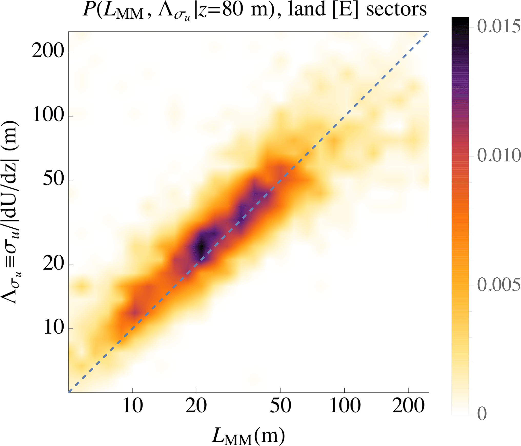
Figure 3Joint probability density function of predicted and diagnosed (observed) turbulent length scale, from measurements at Høvsøre over the homogeneous eastern land sectors. x axis: Mann-model scale L_MM from spectral fits; y axis: L_MM estimated from direct measurements of dU∕dz and σ_u, via Eq. (15).

Download

To demonstrate the statistical character of Eq. (15), as well as its potential for probabilistic use (e.g., as input to probabilistic load calculations), Fig. 4 shows the probability density P(L_MM). As in Fig. 3, L_MM is again calculated from fits to 10 min spectra and also estimated by ${\mathit{\sigma }}_{u,\text{obs}}/(\mathrm{d}U/\mathrm{d}z)$, i.e., Eq. (15). Additionally Fig. 4 displays P(L_MM) for L_MM calculated through Eq. (11), i.e., $c_m{u}_{*}/(\mathrm{d}U/\mathrm{d}z)$; this is done both using the value of c_m=1.7 reported by Peña et al. (2010) as well as using the approximate mean of 2.3 found to be consistent with measurements and theory in Sects. 3.1 and 2.2 above. From Fig. 4 one sees that, for values of turbulent peak scale greater than the mode (∼20 m) up to roughly 150 m, there is a match between the distribution of the diagnosed L_MM and distributions of length scale estimated from the forms (15) based on σ_u,obs and (11) based on u_* with c_m=2.3; these are roughly equivalent for this case over relatively simple homogeneous terrain. It is found that the Peña et al. (2010) value of c_m=1.7 leads to overprediction of L_MM by a factor of 2 or more at scales smaller than 10 m and underprediction by 50 % or more at scales larger than 50 m. The u_*-based form (11) using c_m=2.3 matches the spectrally fit diagnosed distribution P(L_MM) slightly better than the σ_u-based form (15), with predicted peak (mode) values of L_MM being about 3–4 m smaller than the diagnosed peak L_MM.

For the homogeneous land case in Fig. 4 the probability density function of $\mathrm{2.3}{u}_{*,\text{obs}}/(\mathrm{d}U/\mathrm{d}z)$ matches P(L_MM) observed from the spectral fits to within 10 %, over the range 10 m ≲ L_MM≲75 m, and the probability density function of ${\mathit{\sigma }}_{u,\text{obs}}/(\mathrm{d}U/\mathrm{d}z)$ also matches within 10 % over the range 15 m ≲ L_MM≲50 m. This is consistent with the darkly colored 1 : 1 patch evident in Fig. 3 and also shows that Eq. (15) (and also Eq. 11 with c_m=2.3) is sufficient for probabilistic wind load simulations, for two reasons. First, the well-matched range of scales corresponds to the most commonly found L_MM. Secondly, although scales smaller than ∼15 m are not rare (with an occurrence of roughly 1 in 6), they will have a diminishing effect on turbine loads. More specifically, L_MM is more than 70 % likely to fall in the 15–75 m range, i.e., P(15 m $<L_{\text{MM}}<\mathrm{75}$ m)>0.7, and L_MM has more than 86 % likelihood of occurrence between 0 and 75 m, for this homogeneous land case at z=80 m. The relatively common shorter scales correspond to weaker turbulent fluctuations (thus loads), because on average ${\mathit{\sigma }}_{u,\text{obs}}\propto L_{\text{MM}}^{\mathrm{2}/\mathrm{3}}$, as implied by Fig. 1 and Eqs. (9)–(15). Further, turbine loads are less influenced by fluctuations characterized by spatial scales significantly smaller than the blade lengths; thus the error in predicted probability for these shorter scales, and the slight underprediction of the most common L_MM, should not significantly influence probabilistic load calculations relying on site-specific L_MM obtained via measurements and Eq. (15).

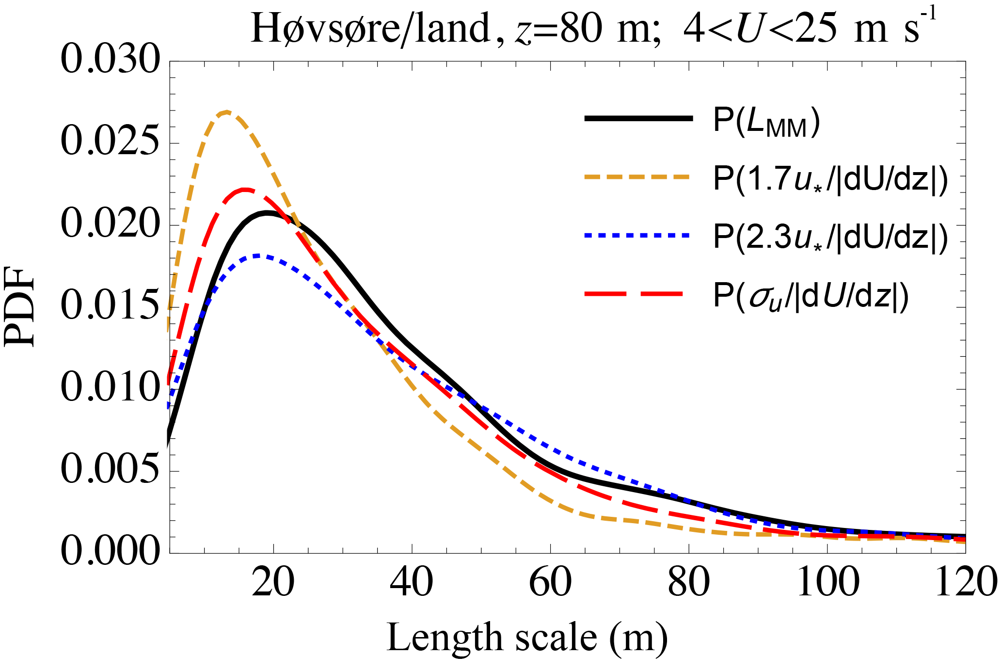
Figure 4Probability density function of turbulent length scale from observations at Høvsøre from the homogeneous eastern land sectors. Black: Mann-model scale from fits to spectra; dotted/blue: “mixing-length” formulation (${\mathrm{\ell }}_m\propto u_{*}/|\mathrm{d}U/\mathrm{d}z|$) with revised constant; dashed/gold: Peña et al. (2010) form for ℓ_m; red/long-dashed: ${\mathit{\sigma }}_u/|\mathrm{d}U/\mathrm{d}z|$ form (15).

Download

While Eq. (15) is useful to estimate L_MM and P(L_MM) as shown above, one expects Eq. (13) to perform better, as it does not rely on the approximation $c_m={\mathit{\sigma }}_u/u_{*}$. Indeed $\langle c_m{u}_{*}/{\mathit{\sigma }}_u\rangle$ is actually 1.11 (or 1.13 if considering winds only down to 7 m s⁻¹) due to ${\mathit{\sigma }}_u/u_{*}$ being slightly smaller and c_m slightly larger than 2.3; using these values in Eq. (13) gives estimates of L_MM closer to the spectrally diagnosed L_MM, and within 10 % of P(L_MM) over a range of L_MM from below 10 m to beyond 100 m. It should also be noted that ignoring speeds below 7 m s⁻¹ can lead to slightly smaller L_MM, since these low wind speeds are more influenced by unstable conditions. Indeed for L_MM≳50 m, including the lower wind speeds causes both diagnosed and predicted L_MM to increase roughly 10 %; this is consistent with larger turbulent eddies being created under unstable conditions.

3.2.1 Estimating P(L_MM) in coastal/offshore conditions

To demonstrate the (probabilistic) use of Eq. (13) or Eq. (15) for L_MM in somewhat different conditions, we now consider flow from offshore, using data from the same mast and height as above (Høvsøre, z=80 m) but for wind directions between 240 and 300^∘. The mast is roughly 1.75 km east of the coastline and subsequently 1.65 km east of a 16–17 m high sand dune that lies 100 m inland, where both are locally oriented in the N–S direction (i.e., for the range of wind directions considered). The dune causes enhanced/accelerated transition of the flow from an offshore (water roughness) to an over-land flow regime (Berg et al., 2015); this results in winds which reflect on-shore and coastal conditions at low heights (below ∼40–80 m depending on stability) and offshore conditions at higher z.

Figure 5 displays the distribution P(L_MM) of spectral-peak (Mann model) length scales for coastal/offshore winds (from west ±30^∘), again using Eq. (15) to estimate L_MM along with L_MM diagnosed through spectral fits. For comparison the corresponding P(L_MM) for easterly winds from Fig. 4 is also included. Just as for the homogeneous land case shown in Fig. 4, one sees in Fig. 5 that, for inhomogeneous coastal conditions, again Eq. (15) gives P(L_MM) basically matching the spectrally fit observations for scales beyond ∼15 m; in this coastal regime the range of well-predicted L_MM extends further, to ∼150 m. While one sees that the distribution of L_MM is a bit different for the (western) inhomogeneous coastal case than for the (eastern) homogeneous land case, the simple expression (15) functions similarly for both flow regimes, with the arguments presented in Sect. 3.2 again applying here.

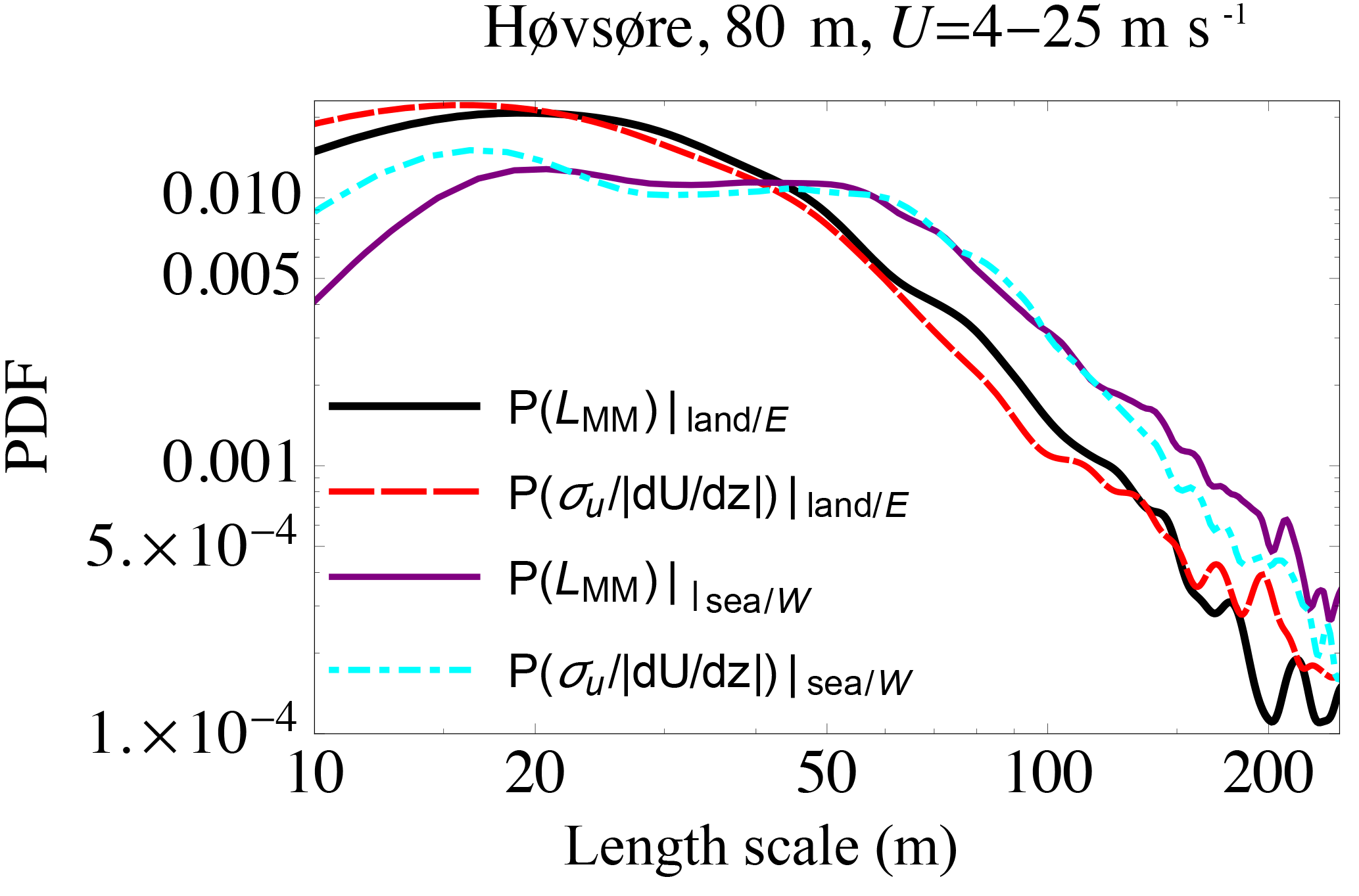
Figure 5Probability density of turbulence length scale L_MM from observations at Høvsøre over both the homogeneous land (eastern) sectors and inhomogeneous coastal (western) sectors. Black: L_MM from fits to spectra over land; red/long-dashed: new simplified form (15) over land; purple: L_MM from fits to spectra from offshore; cyan/dot-dashed: new simplified form (15) from offshore.

Download

The u_*-based Eq. (11) also behaves similarly (not shown) as in the homogeneous land case of Fig. 4, i.e., with gross overpredictions at small scales and underpredictions at large scales. One difference between the coastal and land cases is that, for small L_MM, Eq. (15) overestimates the distribution P(L_MM) a bit more for the coastal regime than for the homogeneous land regime (L_MM<20 m); as explained above for the land case, an overprediction at the smallest scales is not expected to significantly impact load calculations, due to the relatively small length scales involved.

3.2.2 Estimation of P(L_MM) in more complex conditions

To further show the behavior of L_MM and the utility of Eq. (15) at a site with more complex conditions, we examine data from the inhomogeneous forested Danish National Test Centre for Large Wind Turbines site near Østerild in Denmark (Hansen et al., 2014). Here sonic anemometer data are available at heights of 10 and 44 m, with concurrent data from three lidars at $z=\mathit{\{}\mathrm{45},\mathrm{80},\mathrm{140},\mathrm{200},\mathrm{300}\mathit{\}}$ m. In this study we consider data from the site's “western lidar”¹⁰, to measure winds that flow over the forest more than 70 % of the time, where the canopy height is 10–20 m (Hansen et al., 2014; Sogachev et al., 2017). The analysis here uses one year (May 2010–May 2011) of wind speeds U≥5 m s⁻¹ from the lidar at 45 and 80 m heights along with the “fast” (20 Hz) data from the sonic anemometer at 44 m. The shear dU∕dz is measured across 45–80 m; the spectra and subsequent turbulence/Mann-model parameters {$L_{\text{MM}},\mathrm{\Gamma },\mathit{\epsilon }$}, as well as and measured quantities $\mathit{\{}{\mathit{\sigma }}_{u,\text{obs}},u_{*,\text{obs}}\mathit{\}}$, are obtained from the sonic anemometer. The measurements are significantly higher than twice the forest canopy height, and thus above the roughness sublayer (Garratt, 1980; Raupach et al., 1980) and amenable to similarity and mixing-length theory (Sogachev and Kelly, 2016) as well as Mann-model use (Chougule et al., 2015).

Just as Fig. 4 showed for flow over homogeneous land at Høvsøre in Sect. 3, here Fig. 6 displays the probability density of turbulence (Mann-model) length scale L_MM observed via spectral fits at z=44 m for Østerild, along with predictions based on both Eq. (11) via $u_{*,\text{obs}}$ and Eq. (15) via σ_u,obs.

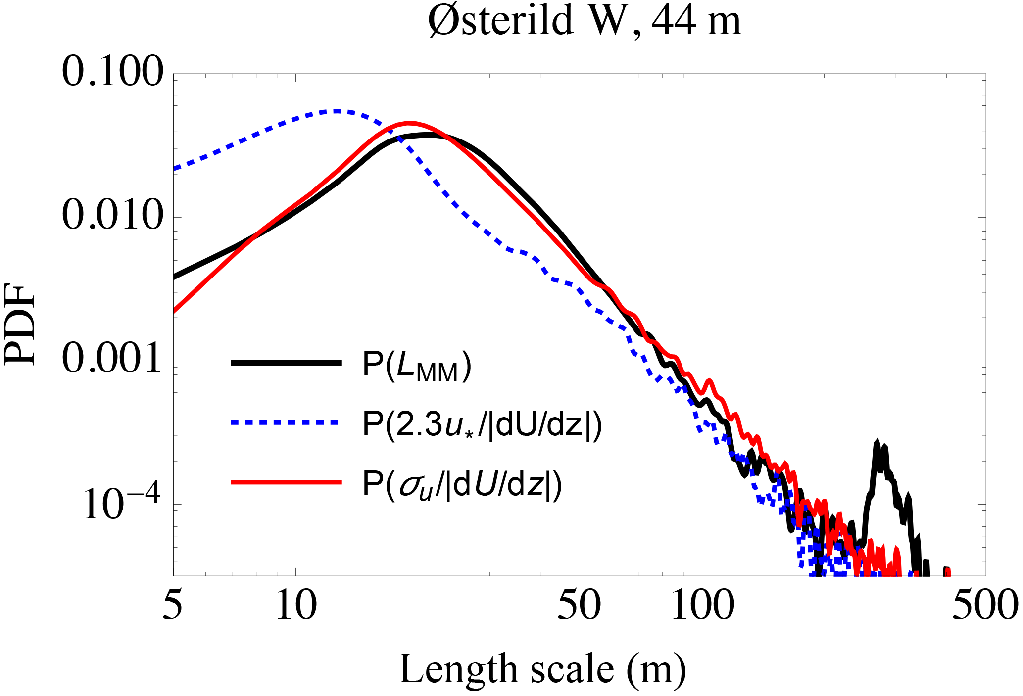
Figure 6Probability density function of turbulent length scale from observations at Østerild from the western mast/lidar. Black: Mann-model scale from fits to spectra; dotted-blue: “mixing-length” formulation (${\mathrm{\ell }}_m\propto u_{*}/|\mathrm{d}U/\mathrm{d}z|$) with revised constant; red: new form (15), ${\mathit{\sigma }}_u/|\mathrm{d}U/\mathrm{d}z|$.

Download

As in the cases above (homogeneous land and inhomogeneous coastal), the new form (15) predicts the distribution rather well, particularly for scales ∼10–100 m – despite the shape of P(L_MM) being different due to the trees. For the forest case of Fig. 6 the σ_u-based form captures both the peak (most likely L_MM) and magnitude of P(L_MM), while the u_*-based form grossly underpredicts L_MM, more so than for the previous cases. The latter is likely due to $u_{*,\text{obs}}$ being predominantly affected by the canopy (via larger effective roughness) more so than σ_u,obs, which tends to be more characteristic of the entire ABL (Wyngaard, 2010). There is, however, a curious minor peak (with a probability ∼1 % as large as the main peak) around scales of $\sim \mathrm{300}\pm \mathrm{50}$ m in the length-scale distribution obtained from spectral fits shown in Fig. 6; this is captured by neither the u_*-based form (11) nor σ_u-based formulations (13) and (15). Although this peak falls spectrally at small wavenumbers that are more difficult to capture when spectrally fitting the Mann model, it actually corresponds to the distance to the next upwind edge of the forest (orchard segment) in the predominant wind directions.

Implications and application

A previously suggested form (11) for L_MM, based on friction velocity u_* and (10 min) mean wind shear dU∕dz (Peña et al., 2010), was confirmed here to be sensitive to its proportionality constant c_m. But this constant can vary from site to site (and possibly with height), and the published value of c_m=1.7 (Peña et al., 2010) leads to significant error in prediction of L_MM for the different conditions (land and sea directions) at Høvsøre and at the forested site of Østerild. Finding c_m from sonic anemometer observations via L_MM from fits to spectra and friction velocity measurements, Eq. (11) may perform slightly better over uniform flat terrain compared to the σ_u-based form (15) – but this can be considered a site-dependent fit in itself, as was the case when using a diagnosed value of c_m=2.3 for the homogeneous flat land sectors at Høvsøre. However, obtaining c_m is generally not possible in industrial practice; where it can be obtained, it relies on L_MM – which is the quantity desired – thus negating the purpose of Eq. (11). While u_* can also in principle be estimated from wind speeds taken at multiple heights by cup anemometers, this too is difficult in practice: one must account for stability, not to mention the need for measurements at multiple heights in the surface layer (or worse, the limited validity of similarity theory above the ASL). Furthermore, it is expected that c_m is a function of the (local) surface roughness, as demonstrated by the different results found over the forested Østerild site. Thus the form (15) is preferable, since it requires only the commonly measured quantities σ_u and dU∕dz. This simple form also gave good estimates of P(L_MM) in the forested case – without the need for tuning, whereas the u_*-based form (11) requires a re-calculation of its coefficient c_m for such cases.

Since Eq. (13) gave yet better performance than both its simplified form (15) and the u_*-based relation (11), one might suggest its use. But Eq. (13) requires $c_m/({\mathit{\sigma }}_u/u_{*})$, where c_m is difficult to obtain, as discussed in the previous paragraph. However, although c_m might vary from site to site (or perhaps with height), it was found that the ratio $c_m/({\mathit{\sigma }}_u/u_{*})$ did not vary appreciably – consistent with the good performance of the simplified form (15), which assumes $c_m\approx {\mathit{\sigma }}_u/u_{*}$, across sites and regimes.

One interesting implication of the testing of assumptions then follows from the finding that $\langle {\mathit{\sigma }}_u/u_{*}{\rangle }_{\text{obs}}\approx \mathrm{2.3}$, consistent in the surface layer with Caughey et al. (1979). Examining the joint behavior of ${\mathit{\sigma }}_u/u_{*}$ and the stability parameter (inverse Obukhov length) L⁻¹, the sonic anemometer data available at multiple heights in this study show no correlation between these two quantities. The dimensionless profiles ${\mathit{\sigma }}_u^{\mathrm{2}}\left(z\right)/u_{*\mathrm{0}}^{\mathrm{2}}$ and $u_{*}^{\mathrm{2}}\left(z\right)/u_{*\mathrm{0}}^{\mathrm{2}}$ shown by Caughey et al. (1979) also imply

with the ratio converging to a constant above the surface layer (z≳0.1h, where the atmospheric boundary-layer depth h typically ranges from ∼200 m in stable conditions to 1 km or more in convective conditions). The flat-terrain Høvsøre data in fact show the mean value $\langle {\mathit{\sigma }}_u/u_{*}{\rangle }_{\text{obs}}$ to be independent of z. If one knew how c_m varied with height (and stability), then one could also use Eqs. (20) and (13) from measurements at one height range, to estimate L_MM at higher z (for a given stability range). Over flat terrain, on average the peak spectral scale for streamwise fluctuations (λ_u) grows with z (Caughey et al., 1979; Peltier et al., 1996)¹¹. Therefore, if we take L_MM∝λ_u, then with Eq. (20) one expects the ratio $c_m/({\mathit{\sigma }}_u/u_{*})$ to increase with z as well. Thus from (13) the Mann-model length scale L_MM will increase with height relative to the mixing length ${\mathrm{\ell }}_{*}\equiv u_{*}/(\mathrm{d}U/\mathrm{d}z)$, so at higher z one would expect the general form (13) to be yet more accurate than its approximate form (15); however, this is not likely for wind turbine rotor heights, except in very stable conditions (Kelly et al., 2014b; Liu and Liang, 2010). Unfortunately the sonic-anemometer measurements available for this study did not include heights well beyond the surface layer, so such variation was difficult to detect.

It is also notable that Fig. 3 appears to imply the relative error (e.g., in %) in estimating L_MM with Eq. (15) grows for less common values of L_MM, particularly very large scales (and also at very small scales if including U<7 m s⁻¹). Thus Eq. (15) is recommended first for estimation of P(L_MM). However, the error at large scales is in part dependent on the limited (10 min) sample lengths and the fitting routine, as there are very few points to fit at the lowest frequencies. Use of 30 min samples can reduce such scatter, and modification of the fitting algorithms may also improve estimations of the larger scales.

Ongoing work includes wind-speed-dependent prediction of L_MM, particularly the conditional statistics P(L_MM|U). Further concurrent work also entails systematic accounting for the rotor size (shear distance) relative to height (i.e., Δz∕z) within the distribution of length scales; following Kelly and Gryning (2010) and Kelly et al. (2014a) a semi-empirical derivation of P(L_MM) including Δz∕z has been obtained but demands more data for validation and publication. Understanding of the latter facilitates “vertical extrapolation” of L_MM and measured turbulence and shear statistics, as well as accounting for the effect of rotor size or shear measurement span.