the Creative Commons Attribution 4.0 License.
the Creative Commons Attribution 4.0 License.
 | 19 Oct 2018
Extending the life of wind turbine blade leading edges by reducing the tip speed during extreme precipitation events
Jakob Ilsted Bech
Charlotte Bay Hasager
Christian Bak
Impact fatigue caused by collision with rain droplets, hail stones and other airborne particles, also known as leading-edge erosion, is a severe problem for wind turbine blades. Each impact on the leading edge adds an increment to the accumulated damage in the material. After a number of impacts the leading-edge material will crack. This paper presents and supports the hypothesis that the vast majority of the damage accumulated in the leading edge is imposed at extreme precipitation condition events, which occur during a very small fraction of the turbine's operation life. By reducing the tip speed of the blades during these events, the service life of the leading edges significantly increases from a few years to the full expected lifetime of the wind turbine. This life extension may cost a negligible reduction in annual energy production (AEP) in the worst case, and in the best case a significant increase in AEP will be achieved.
- Article
(17266 KB) - Full-text XML
- BibTeX
- EndNote


Leading-edge erosion (LEE) is a severe problem for the wind energy sector today (Keegan et al., 2013; Slot et al., 2015). Wind turbine operators report significant costs for inspection, maintenance, repair, and loss of energy production due to downtime and reduced performance (Stephenson, 2011). LEE increases the surface roughness of blades and deteriorates the aerodynamic performance resulting in lower annual energy production (AEP) during turbine operation (Zidane et al., 2016). The LEE issue has appeared as a consequence of the trend towards larger turbines with longer blades and higher nominal tip speeds (Keegan et al., 2013; Macdonald et al., 2016). As an example, recently 273 blades with less than 7 years in operation were refurbished at an offshore wind farm in the North Sea. Some of the blades were even removed and taken ashore for the repair of damages due to LEE (Wittrup, 2015). During the review phase of this paper, it has been revealed that several blades of one hundred and eleven 3.6 MW turbines at the Anholt offshore wind farm will be dismantled and brought ashore for the repair of leading-edge erosion damage less than 5 years after the wind farm was inaugurated. Similar repair campaigns are foreseen for the London array with 175 similar turbines and other UK offshore wind farms (Renews, 2018a, b; OffshoreWind.Biz, 2018).
LEE is caused by a multitude of factors within the atmospheric environment and the leading-edge structure. In addition to rain, impacts of sand particles (Zidane et al., 2017) and other airborne particles such as hail stones (Macdonald et al., 2015) and of insects, global strain from blade flexing, temperature oscillations, UV radiation, and long-term exposure to moisture, chemicals, and salt also add to the material degradation. Efforts to understand rain-induced erosion include simulation (Blowers, 1969; Springer, 1975; Sloth et al., 2015; Amirzadeh, 2017a) and laboratory testing (Bowden et al., 1964; Keegan et al., 2013). A thorough understanding of rain erosion of layered anisotropic polymer-based structures like wind turbine blades is not yet available. However, it is clear that several damage mechanisms are observed and that the impact velocity is a governing factor as well as the amount of precipitation and the structure and materials of the leading edge (Siddons et al., 2015; Cortés et al., 2017).
The industrial standard for measuring the durability of leading-edge structures is the whirling arm rain erosion test (WA-RET) (ASTM G73-10, 2017; Liersch, 2014 – DNVGL-RP-0171). In the WA-RET the test specimens are mounted on a rotor spinning at high velocity in an artificially generated rain field. The rotor velocity, rain intensity, and droplet size are carefully controlled, as impact velocity, droplet dimension, and the number of impacts are the governing factors for the magnitude of damage imposed on a given test specimen (Adler, 1999). It should be kept in mind that the whirling arm test method does not reflect the real operating conditions for rain impact. The impact velocities of the accelerated tests are typically up to 2 times the tip speed of real blades, which may cause irrelevant failure modes. Also, the fixed rain field with constant rain intensity and drop size distribution is very different from field conditions, where droplet sizes and rain intensity vary a lot (Best, 1950).
Blade and turbine manufacturers as well as coating suppliers put effort into developing and implementing leading-edge protection structures that will last the expected lifetime of the turbines. Wind turbine (WT) operators put effort into defining feasible inspection and service intervals and into repairing damaged blades. The latest developments in leading-edge protection (LEP) applied to new turbines have yet to prove their durability in long-term field conditions. Already installed turbines without the latest inventions in LEP are still vulnerable to erosion, and repairs made on-site may have varying quality. Also, in order to reduce the torques and loads, it may be attractive to increase the tip speeds even further on future turbine designs. Consequently, alternative strategies of the mitigation of LEE should be explored.
Such an alternative strategy is the reduction in the tip speed during highly erosive conditions (Wobben, 2003). It is likely to be feasible to extend the leading-edge life by reducing the rotor speed during extreme precipitation events occurring at a very small fraction of the service life but accounting for the majority of the erosion damage. The threshold values of precipitation as an indicator of tip speed reduction will be determined for the individual wind turbine plant as described in Sect. 5. The approach to erosion control is inspired by aerodynamic load control, where it is a common strategy to reduce the extreme loads caused by gusts and turbulence by pitching out the blades under these conditions. Such systems operate automatically in modern wind turbines (Njiri et al., 2016).
The objective of this paper is to present and support the hypothesis on the mitigation of leading-edge erosion by control of wind turbines during high-intensity rain events. In Sect. 2 some important aspects of leading-edge erosion are presented with a focus on liquid droplet impact stresses and fatigue. Section 3 presents an analysis of whirling arm rain erosion test data provided by PolyTech A/S. The analysis includes an introduction to block loading and a cumulative damage law. Section 4 presents precipitation parameters and their statistical occurrence, while Sect. 5 focuses on turbine control for reducing tip speed and includes control strategies with different degrees of loss of production vs. extension of the life of blades. The discussion follows in Sect. 6, and conclusions are drawn in Sect. 7.
2.1 Droplet impact
Rain erosion is the consequence of multiple impacts stochastically distributed over the surface of the coated laminate. Each impact adds a damage increment to the accumulated damage. For rain and other airborne particles the accumulated damage is a function of several parameters including the number of impacts per unit area, and the magnitude of each impact. This paper is limited to considering the impact by liquid droplets only.
The magnitude of an impact of a droplet hitting perpendicular to the surface may be quantified by the kinetic energy (Ek):
where v is the velocity of the particle relative to the surface and m is the mass of the droplet.
For detailed analysis the impact may be quantified by the contact stress field acting on the surface as a function of time during the impact (Keegan et al., 2012). The contact stresses are functions of the properties of the liquid, the properties of the impacted surface, the impact velocity, and the size and shape of the droplet.
The impact of a spherical droplet immediately causes a normal pressure on the target surface at the initial point of contact. The contact area between the droplet and the solid expands radially at a velocity higher than the speed of sound in water. When the shock wave front reaches the edge of the droplet, a release jet is generated, and the pressure reduces to the stagnation pressure (Bowden, 1964; Dear and Field, 1988).
The simplest expression for the calculation of the initial contact pressure is the water hammer equation (Bowden, 1961). It was derived for a column of liquid impacting a rigid surface, where a compression wave propagates from the contact into the liquid. The immediate contact pressure (p) may be calculated by
where v is the impact velocity, cl is the speed of the compression wave in the liquid, and ρl is the density of the liquid. Accounting for the geometry of a spherical droplet, the contact angle increases as the contact area expands, and the peak pressure at the rim of the contact is analytically derived (Heymann, 1969) as
Taking into account the compliance of the solid, the pressure of the impact between an elastic solid cylinder and a liquid jet (de Haller, 1933) may be expressed as
where subscript “l” is for liquid and “s” for solid. Later numerical modelling works take into account an assumed spherical geometry of the droplet as well as the compliance of the target material (Adler, 1995; Amirzadeh et al., 2017b). These studies also show a pressure peak near the edge of the contact.
Real precipitation droplets falling through the atmosphere are not necessarily spherical. The aerodynamic forces distort the droplet to a burger-bun-like shape. Larger droplets, d > 6 mm, flatten out before splitting up (Fakhari, 2009), while smaller droplets tend to merge and form larger droplets. The droplet geometry may be characterized by its ratio of vertical to horizontal dimensions (Gorgucci et al., 2006). Through a full rotation of 360∘, the wind turbine blades are hitting the non-spherical droplets from all angles at different relative velocities. This makes the impact scenario even more complex.
2.2 Impact stresses, fracture and fatigue
A typical leading edge consists of a curved laminate of glass-fibre-reinforced polymer (GFRP) with a relatively brittle polyurethane-, polyester- or epoxy-based coating. Many designs have a layer of putty or filler, applied to the laminate and sanded, to make a smooth surface for the coating. Recent developments have added a top layer of elastomeric coating with good damping properties and high fracture toughness, often referred to as leading-edge protection or LEP; see Fig. 1 (taken from Cortés et al., 2017).
An impact on the surface causes stress transients in the material. Stress waves propagate from the impact site into the coated composite (body waves) and along its surface (surface waves). Several stress components are active as functions of the time after the impact, the radial planar position and depth in the material (Woods, 1968; Adler, 1995). These stresses can activate different failure modes depending on the velocity of the impact, the size of the droplet and “the weakest link” in the leading-edge structure.

Figure 1Example of leading-edge protection system configuration (Cortés et al., 2017).
For isotropic, homogenous, elastic materials ring-shaped surface cracks due to Rayleigh waves are the common type of impact damage (Blowers, 1969; Bowden, 1964). For many coated materials, this may also be the governing failure mechanism.
The body waves propagating perpendicular to the surface into the target material can lead to subsurface cracks in the coating and the substrate (Fraisse et al., 2018). The reflection of stress waves between the coating surface and the coating–substrate interface may also play a significant role in the fatigue of the coated laminate (Springer, 1974). Body waves may also cause delamination inside the laminate (Prayago, 2011) and debonding of the coating (Cortés et al., 2017).
A single droplet impact may cause instant damage when the impact velocity is beyond the damage threshold velocity (DTV). For a given droplet size and set of material parameters, DTV was derived for brittle materials by a fracture mechanics approach (Evans et al., 1980).
where Kc is the critical stress intensity factor, cs is the Rayleigh wave velocity of the target material, D is the diameter of the spherical droplet, ρl is the density of the liquid, cl is the speed of sound in the liquid and λ is a material independent constant.
Repeated stresses below the static strength of a material may eventually cause failure due to cumulative fatigue damage (Miner, 1945). Similarly, impacts below DTV may also add to the accumulated damage, which may eventually cause fracture (Springer, 1975). For materials with a fatigue limit, like some metals, a fatigue threshold impact velocity, below which no erosion will occur, may be defined as an analogy to the endurance limit found in fatigue testing (Heymann, 1969). Rain erosion test data can be regarded as impact fatigue data. Together with operational data for a wind turbine and the local precipitation statistics, it can be used to predict the erosion propagation and lifetime of leading edges in field operation (Eisenberg et al., 2016).

Figure 2Whirling arm rain erosion test specimen photographed at 30 min intervals during 3 h of testing.
3.1 Analysis of rain erosion test data
An example of rain erosion test data was made available by PolyTech A/S; see Fig. 2. The test specimen material is coated aluminium. The specimen has a length of 225 mm. In this test, the tangential velocity was 140 m s−1 at the tip and 110 m s−1 at the root of the specimen. The rain intensity was 30–35 mm h−1, and droplet sizes ranged from 1 to 2 mm. In the later calculations, for simplicity, it is assumed that the rain intensity is 32.5 mm h−1, and the droplet diameter is uniform at 2 mm. The falling velocity of the droplets is assumed to be 6 m s−1, corresponding to the terminal velocity of 2 mm droplets (Foote et al., 1969). The test was stopped every 30 min for photography of the specimens; see Fig. 2. The photographs are used to determine the progression of erosion. Here, erosion is defined as the visible removal of the top coat. The erosion initiates at the tip of the specimen, where velocity is highest. It then propagates towards the root, where the velocity is lower. Each position on the specimen corresponds to a certain tangential velocity. The data pairs of the position of the erosion front and the time are shown in Table 1 along with the corresponding local rotor velocities. The kinetic energy of each impact and the number of impacts per unit area are explained in Sect. 3.2.
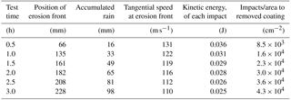
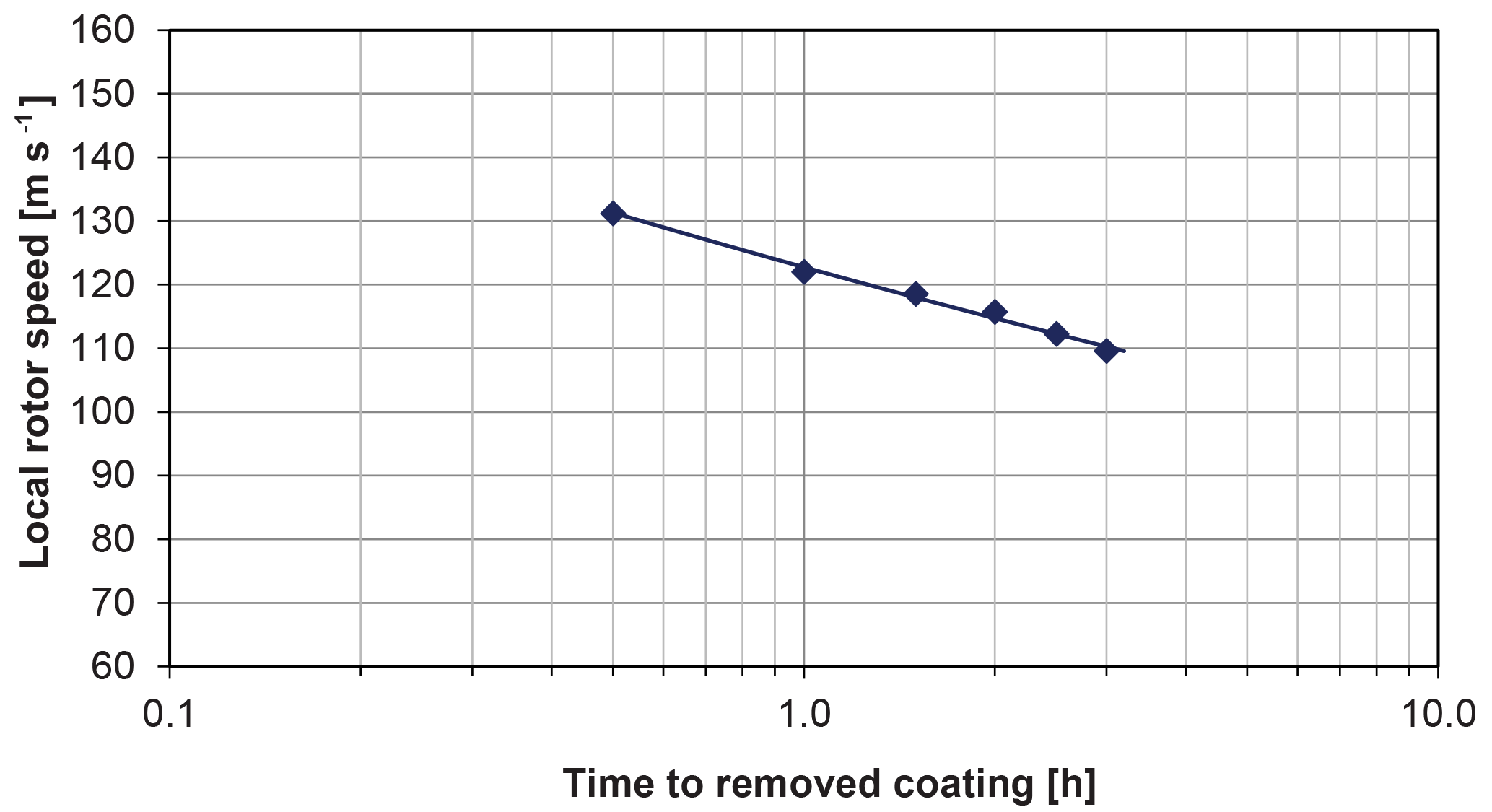
The data on time to removed coating as a function of the local rotor speed from Table 1 are plotted in Fig. 3
Rain erosion can be analysed as a fatigue process (Slot et al., 2015), where, traditionally, the independent parameter, here velocity, is plotted on the vertical axis and the dependent parameter, here the time before the coating is removed, is plotted on the horizontal axis of a semi-logarithmic diagram.
3.2 Generalizing empirical values
Exactly how the droplet sizes and velocities influence the damage is unknown. It obviously depends on several factors including material configuration: properties of coating, putty and laminate, layer thicknesses, interfaces, and various failure modes. We now take the hypothesis that the kinetic energy of each impact characterizes the magnitude of the impact and that the number of impacts per square centimetre corresponds to the number of cycles in a fatigue test.
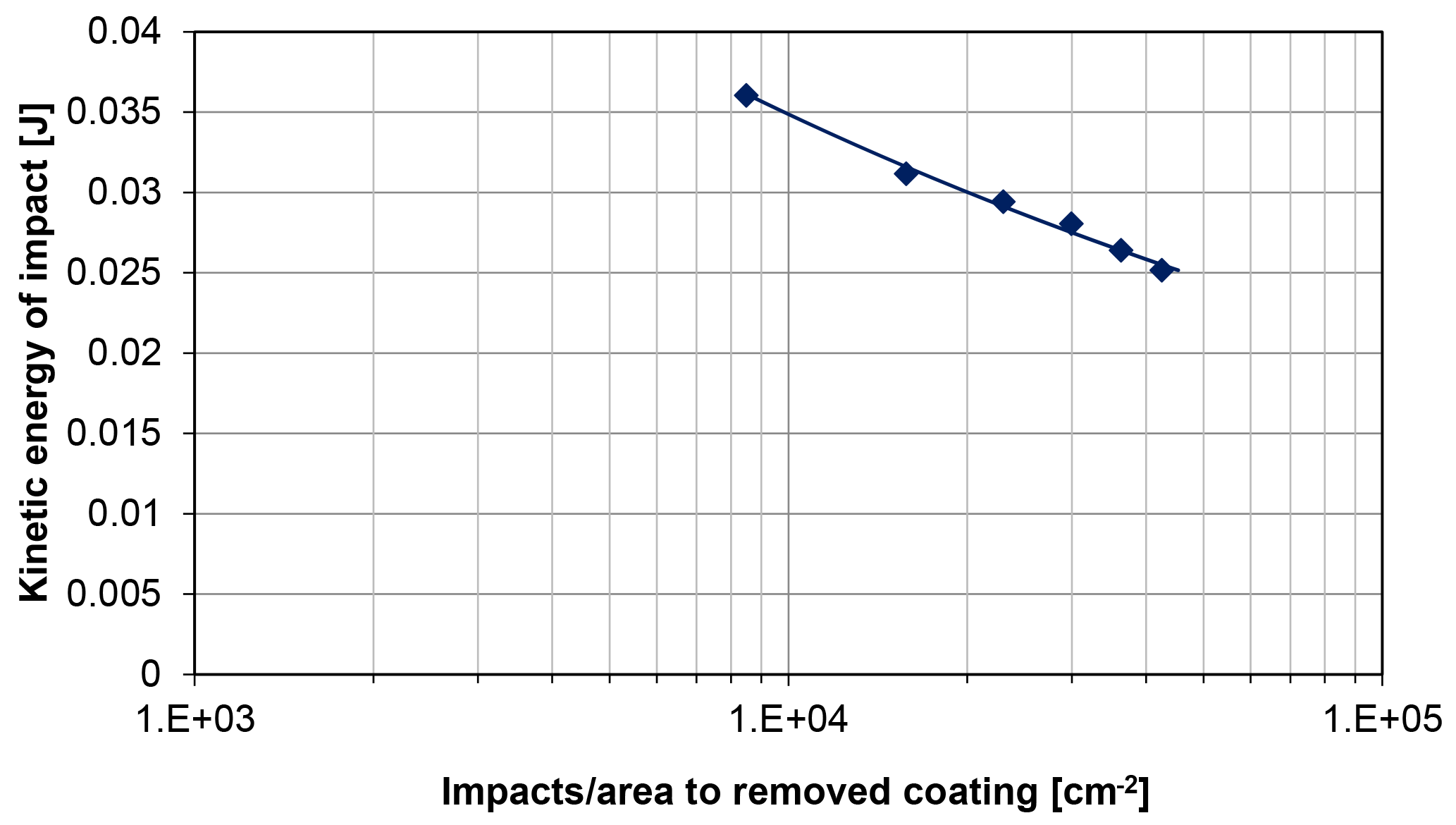
Figure 4Rain erosion test data plotted as a Wöhler curve: impacts per unit area to failure as a function of the kinetic energy for each impact.
For an object travelling through a rain field with assumed spherical droplets with uniform diameter and constant falling velocity, the impact frequency can be calculated analytically (Gohardani, 2011; DNVGL, 2018).
The relative volume of water in the rain field, V, is given by
where Ir is rain intensity and vr is falling velocity.
The number of droplets per volume, N, can be expressed as
where D is droplet diameter.
An object travelling through a rain field is hit by droplets in a stochastic manner across its surface. Assuming that the droplets are distributed evenly in space and their velocity is negligible compared to the speed of the object, the impact frequency or the number of impacts per unit projected area per time, F, can be expressed as
The kinetic energy, Ek, of each impact is
Now, the test data from Table 1 can be presented as the number of impacts per unit area, NEi, as a function of the kinetic energy of each impact before the coating is removed; see Fig. 4. Such a representation of data, often referred to as a Wöhler curve or SN curve, is known from fatigue testing of materials (Miner, 1945; Ronold and Echtermeyer, 1996), where the number of load cycles causing failure is shown as a function of the magnitude of each load cycle (for example stress range). Fatigue data are often fitted to a power function as shown in Fig. 4.
E0= 1 J. A power function fit of the test data in Table 1 to Eq. (10) gives c=18 and m=4.63
We now take the additional hypothesis that the incremental damage is a function of the impact energy only and that Eq. (10) holds for different droplet diameters.
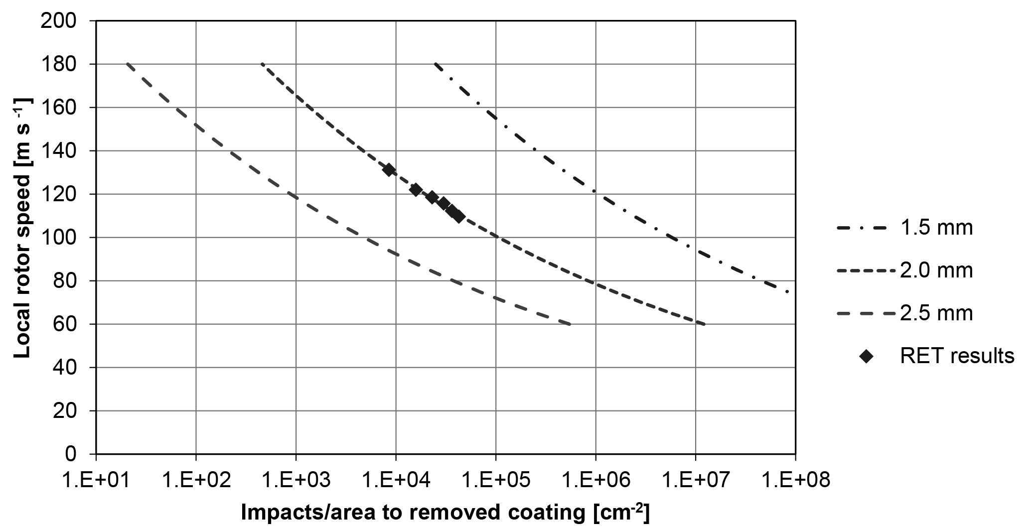
Combining Eqs. (9) and (10), the fatigue life can be expressed as a function of the impact velocity and the droplet diameter:
Now, applying Eq. (11), Wöhler curves can be drawn for different droplet diameters as shown in Fig. 5.
Back-calculating from impacts per area to millimetres of accumulated rain, one gets the Wöhler curves for accumulated rain to remove the coating as a function of the rotor velocity for different droplet diameters as shown in Fig. 6.
Given the assumptions and extrapolation, it is obvious that droplet size is important and not just the amount of rain.
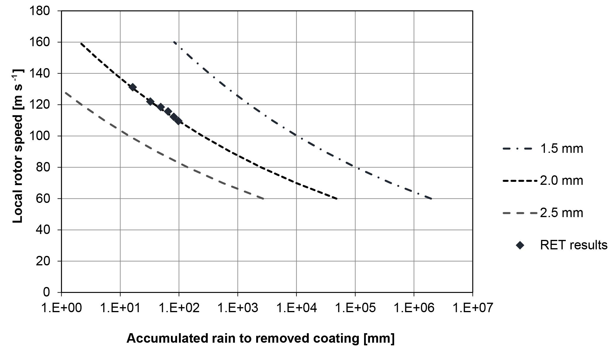
Figure 6Expected accumulated rain to remove coating as a function of rotor speed for droplet diameters of 1.5, 2.0 and 2.5 mm.
3.3 Block loading and cumulative damage laws
Each point on the Wöhler curve in Fig. 3 corresponds to a test run at constant conditions (rain intensity, droplet size, local rotor speed). However, most structures designed for cyclic loads are subject to varying load intensities in service. For instance a wind turbine blade will see a spectrum of wind speeds, gusts and turbulence over its lifetime. Likewise, a leading edge will be impacted with rain of varying droplet sizes and intensities and changing impact velocities. To account for variable-conditions fatigue loading, different rules have been proposed for the accumulation of damage in composites (Brøndsted et al., 1997). The most popular and easy to use, though not always correct, is the linear Palmgren–Miner rule. Accumulated damage (M) is given by
Here, i is the load level number, ni is the number of cycles at level i, Ni is cycles to failure at level i in a test and j is the number of load levels. The expected fatigue life of a cyclic loaded material is reached when M≥1.

Figure 7Raindrop size distribution through a horizontal plane with the rain fall intensity as a parameter (from Kubilay et al., 2013, based on Best, 1950).
Given a load time history and Wöhler curves for different loading conditions, it is possible to use Miner's rule to determine the accumulated damage or fatigue life of a structure or material. The Palmgren–Miner rule has been used to predict the rain droplet impact fatigue life of a leading edge (Slot et al., 2015; Amirzadeh et al., 2017b). Here, it will be applied later to predict the fatigue life of a leading edge based on the presented rain erosion test (RET) data and rain statistics.
Estimation of the potential erosion caused by rain at specific wind farm sites has to be based on information on precipitation, wind speed and turbine characteristics such as tip speed. Wind speeds at wind farm sites are usually known from wind resource assessment during the planning phase and on-site wind observations during the operational phase. In contrast, precipitation is not a standard observation, neither for planning nor for operating wind farms.
Early studies on raindrop size distribution (Best, 1950; Mason and Andrews, 1960) showed rain intensity and raindrop size to relate to each other for a wide range of climate conditions. Figure 7 shows the probability density function as a function of raindrop diameter for six rain intensities ranging from 0.1 to 20 mm h−1 based on Best (1950) (Kubilay et al., 2013).
Rain intensity (or rate) is typically measured as millimetres per hour. Rain intensity varies a lot with time. The shorter the interval of measurement the more detailed is the picture of variation.
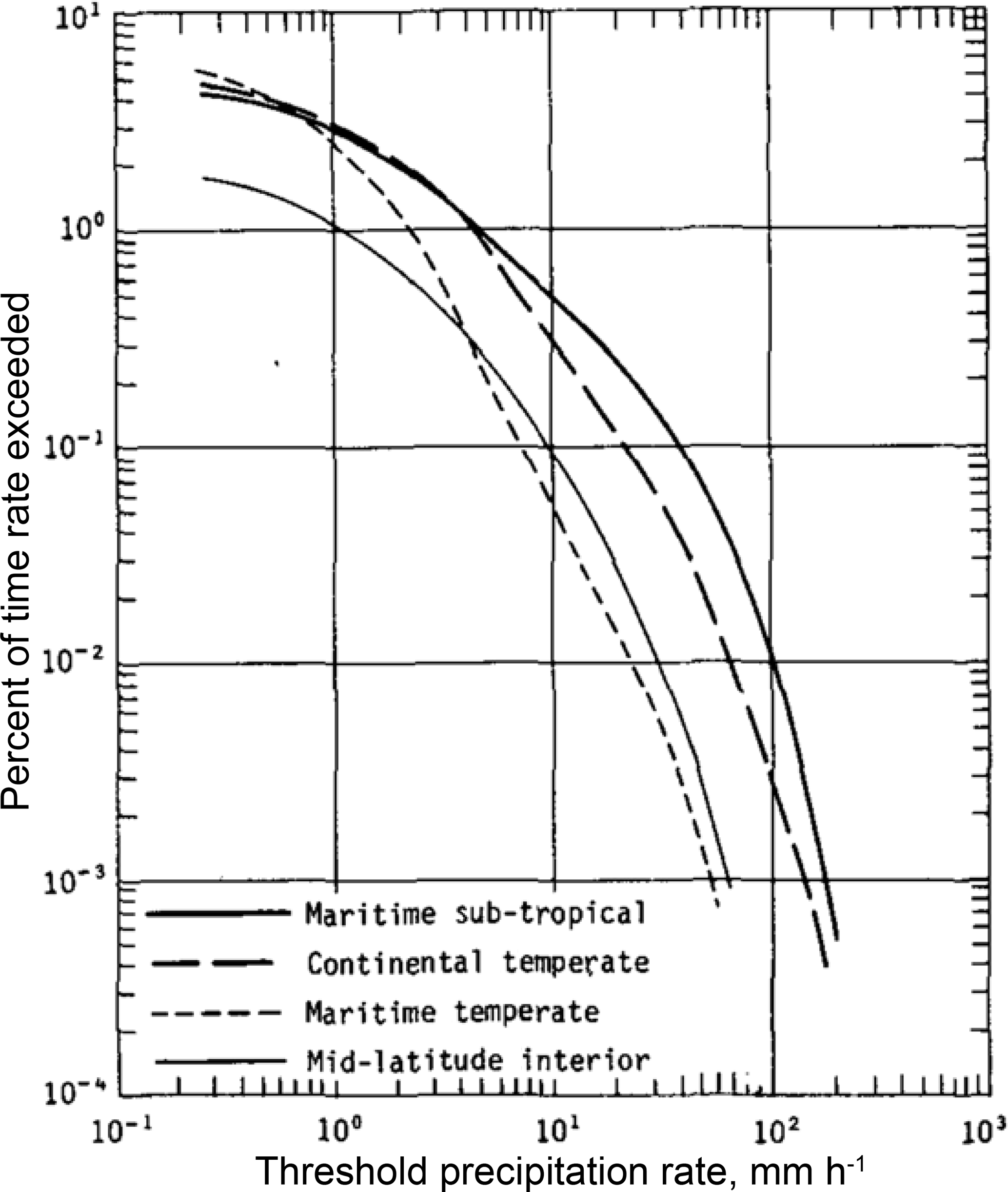
Figure 8Average rainfall-rate–frequency relationships for four rain climates (Jones and Sims, 1978) American Meteorological Society©. Used with permission.
Based on disdrometer observations in New Jersey, USA, Smith et al. (2009) showed that raindrop size distribution and rainfall intensity in heavy convective rain can be described from a Γ distribution. For a convective rain event, the rain intensity at 1 min intervals can be more than 10 times higher than the intensity measured at 60 min intervals, (Smith et al., 2009). Convective rain is a type of precipitation, which is generally more intense, and of shorter duration, than rain from larger weather systems.
Similar results are found in tropical rainfall during the monsoon season in Malaysia (Hong et al., 2015). Precipitation measured by disdrometers at locations across the globe from Australia and Asia to Europe and America confirm the relationship between rain intensity and raindrop size distribution (Bringi et al., 2003). Interestingly, Bringi et al. (2013) distinguish between convective “maritime” and convective “continental” raindrop size distributions with the first being characterized by a lower concentration of larger-sized drops as compared to the latter. The generalization on average rainfall rate and the percentage of time of exceedance for different rain climates is shown in Fig. 8 (Jones and Sims, 1978). Figures 7 and 8 are used for input to droplet sizes and rain intensities for the simplified rain climate statistics used in Sect. 5.1.2, Tables 4 to 8.
Precipitation varies much across the globe. Mean annual precipitation and the monthly mean precipitation during the driest and wettest months are used in the Köppen–Geiger climate classification (Peel et al., 2007). The climatological standard normal covers 30 years according to the world Meteorological Organization. The mean annual precipitation normal is based on local network station records on land and varies much spatially. Table 2 lists data from Scandinavia, the UK, Europe and the world. The wettest place on Earth is said to be in India with 11.871 mm yr−1 (source: World Atlas).
Table 2Mean annual precipitation ranges over land in selected countries, Europe and the world. FMI: Finnish Meteorological Institute; Met. no: Norwegian Meteorological Institute; SMHI: Swedish Meteorological and Hydrological Institute.

NA: not available.
Precipitation over the ocean is mapped mainly by Earth observing satellites and to lesser degree based on sparse observations from ships and weather stations on small islands. The annual precipitation during the years from 1998 to 2011 observed by the Tropical Rainfall Microwave Mission (TRMM) between latitudes 40∘ N and 40∘ S is shown in Fig. 9. The spatial resolution is 0.25∘ by 0.25∘. Annual rainfall up to 7300 mm is noted in some tropical regions over the ocean. Over land the TRMM map shows dry and wet regions corresponding to precipitation maps based on weather stations.

Figure 9Average rainfall measured by TRMM from 1998 to 2011. Source: NASA (2018).
The global precipitation map covering the years from 1988 to 2004 is shown in Fig. 10. This map is based on the Special Sensor Microwave Imager, the GOES precipitation index, the outgoing longwave precipitation index, rain gauges, and sounders on NOAA satellites (source: Global Precipitation Climatology Project (GPCP); http://gpcp.umd.edu, last access: 11 September 2018). The spatial resolution is 2.5∘ by 2.5∘. The map shows that annual precipitation is above 3300 mm yr−1 over the ocean in some tropical regions. It may be noted that this spatial resolution does not resolve details. The maps for Scandinavia, the UK, Europe and the world listed in Table 2 do not cover the sea. TRMM only covers between 40∘ N and 40∘ S. Thus, a map of the 30-year mean annual precipitation in the northern European seas, where the majority of offshore wind farms are located, is not available (to the knowledge of the authors).

Figure 10Average rainfall measured by several satellites, sounders and rain gauges combined for the years 1988 to 2004. Source: GPCP (2018).
The objective to estimate the potential erosion caused by rain at specific wind farm sites is obviously more challenging at sea than at land due to the limited available precipitation data. Over land the rainfall erosivity for soil degradation has been assessed from weather station data (Panagos et al., 2015, 2017). It is based on the Revised Universal Soil Loss Equation (RUSLE) method (Naipal et al., 2015). Rainfall erosivity is modelled as a function of the kinetic energy of rain, the maximum intensity of rainfall, the cumulative rainfall, the soil properties and the slopes of terrain. The map on rainfall erosivity in Europe at 500 m spatial resolution assessed by European Soil Data Centre (ESDAC) is shown in Fig. 11 (Panagos et al., 2015). A comprehensive precipitation database has been established (Panagos et al., 2015, 2017). This database would be valuable for the production of a rain erosion map for wind turbines where precipitation, wind speed and turbine characteristics such as tip speed would be input.
For offshore wind farms the leading-edge life is significantly shorter, than what is observed on land due to longer blades and higher tip speeds offshore (Cortés et al. 2017) and likely also due to offshore rain and wind conditions, ocean salinity, and marine air composition. The wind turbine blades offshore need inspection and repair during their lifetime. The access to offshore wind farms is dependent upon suitable weather conditions, and the cost of keeping staff and machinery waiting for the right weather window can be significant (Poulsen et al., 2017). During repair with leading-edge protection on offshore blades, the weather window requires benign wind and waves plus air temperatures above 15 ∘C, relative humidity < 60 % and no warning for thunderstorm and lightning. In the northern European seas this limits repair campaigns to the summer period. It may be valuable to assess the likelihood of suitable weather windows, in addition to the wind resource and the potential rain erosion for improved overall assessment of lifetime cost for offshore wind farms.
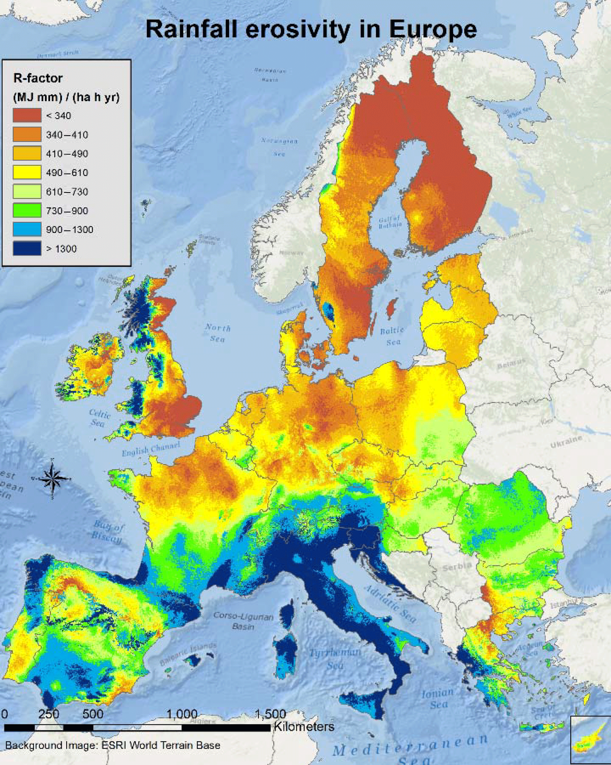
Figure 11Rainfall erosivity in Europe at 1 km grid cell resolution. Source: Panagos et al. (2015). Creative Commons Attribution-NonCommercial-NoDerivatives License (CC BY-NC-ND, https://doi.org/10.1016/j.scitotenv.2015.01.008; last access: 11 September 2018).
Leading-edge erosion causes an increase in surface roughness of the blade and thereby an increase in the air flow boundary layer thickness over the airfoils on the blade when it is operating. The increased boundary layer thickness causes an increased drag coefficient and a decreased lift coefficient, and thus reduces the aerodynamic performance, particularly at higher angles of attack (AOA) (Sareen et al., 2014). The consequence is severe losses in energy production. To investigate the influence of the erosion on the aerodynamic performance and on the AEP, aerodynamic rotor computations were carried out for a Vestas V52 wind turbine with a modified control system. First, the method is described, and then the results are shown.
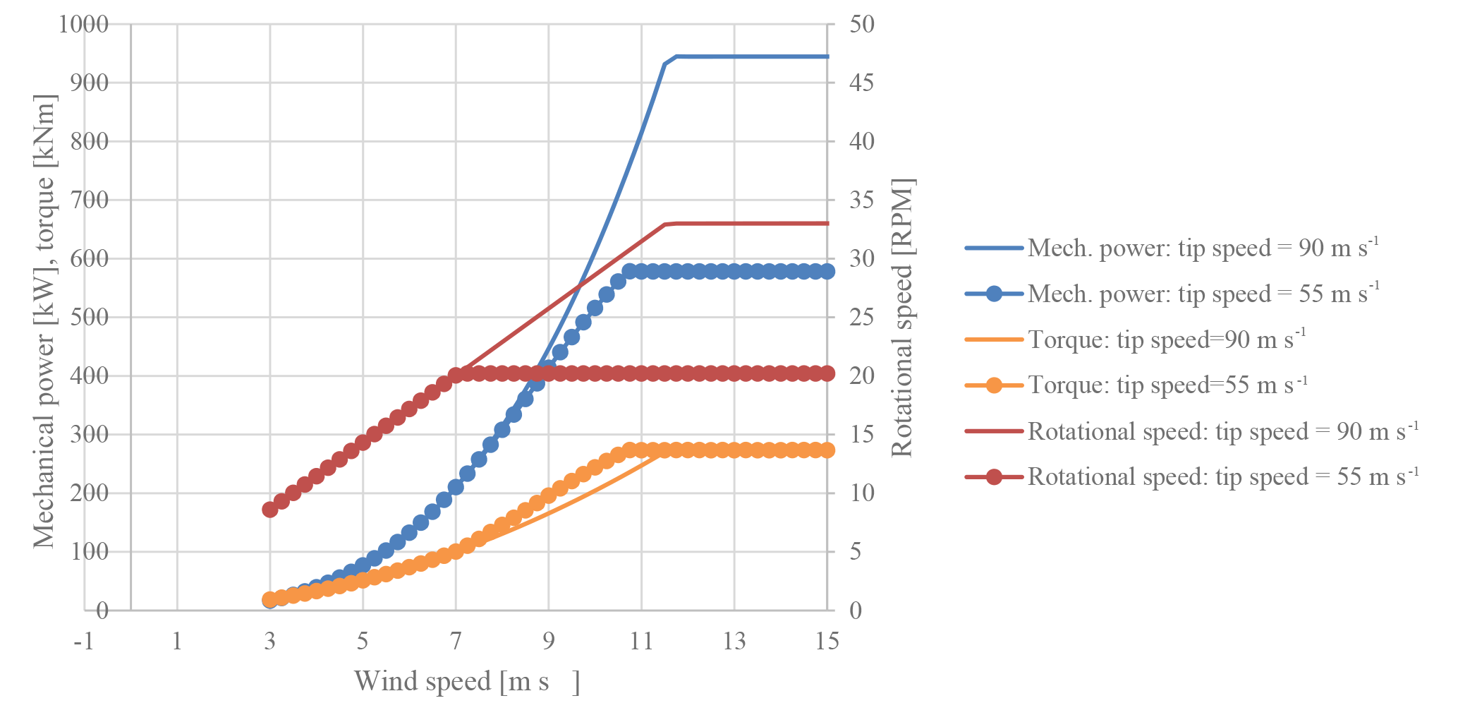
Figure 12Mechanical power, rotational speed and main shaft torque as functions of wind speed for control of the rotor with maximum tip speeds of 90 and 55 m s−1.
5.1 Methods
5.1.1 The wind turbine
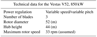
The investigation was carried out as simulations on the Vestas V52 850 kW pitch-regulated variable-speed wind turbine that was erected at the DTU (Technical University of Denmark) Risø Campus during the summer of 2015 (Table 3). This wind turbine was chosen because data were available. However, parts of the input were modified; for example, this was done for the rotational speed to make it consistent with the higher tip speeds that modern wind turbines are designed with. The size of the wind turbine is somewhat smaller than the majority of wind turbines installed during the last decade, but the relative losses in annual energy production are considered similar. The simulations were carried out assuming steady state, no yaw and no aeroelastic response. These assumptions simplified the conditions significantly but were made to investigate the main response. A further description of the simulations is found in Sect. 5.1.3 to 5.1.5.
5.1.2 Control of the wind turbine
The wind turbine control is of the pitch-regulated variable-speed type. The maximum tip speed is assumed to be 90 m s−1 and is thereby greater than the tip speed of an original Vestas V52 wind turbine. Compared to common control strategies, this wind turbine is assumed to have a precipitation sensor. The sensor is capable of measuring and giving input to the turbine controller regarding the present rain intensity and/or the droplet size. As the tip speed is a governing factor in the erosion rate, the erosion control strategy consists of reducing the maximum tip speed when the rain intensity and droplet size exceed threshold values. This is done by reducing the maximum rotational speed of the wind turbine. Because a wind turbine is designed for maximum torque in the drive train, the reduction in the rotational speed implies that the maximum power is reduced. The wind turbine with the original control can produce a maximum mechanical power described by , where P0 is the original rated mechanical power, Q0 is the original rated main shaft torque and ω0 is the original maximum rotational speed. When reducing the rotational speed from ω0 to ω1, the maximum torque limit must not be exceeded. Then the maximum power is also reduced to P1 (). An example from the computations is shown in Fig. 12. It is seen that the maximum torque is maintained despite the difference in maximum rotational speed.
Five different erosion control strategies (ECSs) are investigated. An ECS is a set of one or more precipitation intensity threshold values and the corresponding maximum allowed tip speeds, (max tip speed at rain intensity threshold). The expected lifetime for the blade leading edge for each ECS is calculated using the droplet-size-dependent Wöhler curves (Eq. 11), the Palmgren–Miner rule (Eq. 12) and the assumed rain data, which are deduced from Figs. 7 and 8 and shown in the columns 1, 2 and 3 of Tables 4 to 8. Additionally a reference case is included, where it is assumed that no erosion occurs.
-
ECS 1: no tip speed reduction; expected lifetime of 1.6 years;
-
ECS 2: 70 m s−1 at 20 mm h−1; 80 m s−1 at 10 mm h−1; expected lifetime of 10 years;
-
ECS 3: 60 m s−1 at 20 mm h−1; 70 m s−1 at 10 mm h−1; expected lifetime of 24 years;
-
ECS 4: 60 m s−1 at 20 mm h−1; 70 m s−1 at 10 mm h−1; 70 m s−1 at 5 mm h−1; expected lifetime of 54 years;
-
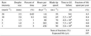
ECS 5: 55 m s−1 at 20 mm h−1; 65 m s−1 at 10 mm h−1; 70 m s−1 at 5 mm h−1; expected lifetime of 107 years;
-
Reference Strategy 6 with no tip speed reduction and an expected lifetime of infinitely many years.
Table 4Calculation of the expected lifetime of the blade leading edge with no reduction in the tip speed. Control Strategy 1.
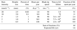
The results of the five first control strategies are shown in Tables 4 to 8. For the Reference Strategy 6, it is assumed that no erosion will occur. The rain intensity frequencies are based on precipitation data for maritime temperate climate from Fig. 8. The fixed droplet sizes for each rain intensity are assumed based on Fig. 7. The expected lifetimes are calculated applying Eqs. (11) and (12) and extensive extrapolation as described in Sect. 3 of the RET data shown in Table 1. The control strategies are based on an assumed behaviour that there is a correspondence between the surface roughness height and the aerodynamic performance. Thus, there are elements in this analysis that are not documented but are based on qualified assumptions. However, the numbers are believed to be sufficiently realistic to demonstrate the potential of erosion control.
Table 5Calculation of the expected lifetime of the blade leading edge with a reduction in the tip speed to 70 and 80 m s−1: Control Strategy 2.

The first row in Table 4 is explained here: the probability of rain intensity of 20 mm h−1 with 2.5 mm droplets is around 0.02 % or 1.8 h yr−1. At this rain intensity the total expected lifetime before failure of the leading edge (LE) at 90 m s−1 is around 3.5 h. The fraction of damage per year relative to LE failure at this level is 51 %. Summing up the fractions of damage per year at the five different rain intensities gives 0.64 % or 64 %. The calculated expected blade LE life at these conditions is therefore year.
Table 6Calculation of the expected lifetime of the blade leading edge with a reduction in the tip speed to 60 and 70 m s−1: Control Strategy 3.
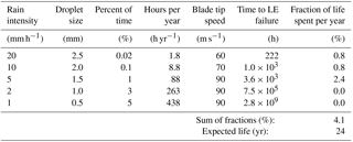
The results in Table 5 show the effect of reducing the tip speed to 70 and 80 m s−1 at the two heaviest rain intensities. Because of the reduction in tip speed the blade life is extended to 10 years. In Tables 6 to 8 the results are shown where a further increase in lifetime is obtained.
Table 7Calculation of the expected lifetime of the blade leading edge with a reduction in the tip speed to 60, 70 and 70 m s−1: Control Strategy 4.


Figure 13Airfoil characteristics of the outer part of the blade: blue – clean blade; red – full leading-edge roughness; green – 60 % of full leading-edge roughness. (a) Lift coefficient, clift, as a function of drag coefficient, cdrag. (b) Lift coefficient, clift, as a function of angle of attack (AOA).
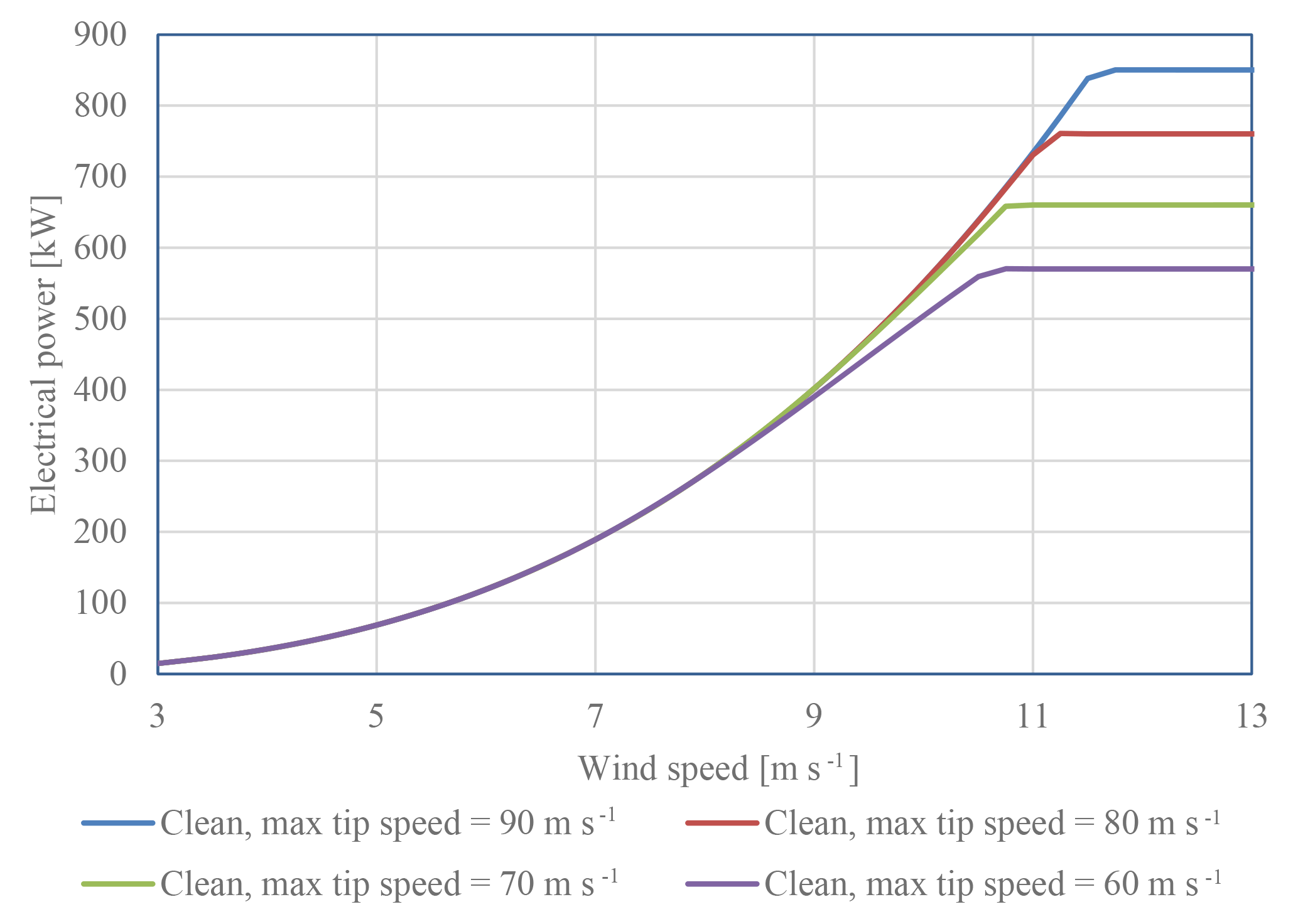
In order to avoid overloading the drivetrain, care was taken not to exceed the maximum rated shaft torque. Thus, when operating at different maximum tip speeds, the wind turbine had to operate at different rated power:
-
90 m s−1: 850 kW;
-
80 m s−1: 760 kW;
-
70 m s−1: 660 kW;
-
65 m s−1: 615 kW;
-
60 m s−1: 570 kW;
-
55 m s−1: 520 kW.
Even though the wind turbine experiences heavy rain and has to reduce the tip speed, the wind turbine will produce some power; thus, only part of the potential power is lost. On the other hand, by using the erosion-safe mode, the repair and loss in production due to leading-edge erosion will be reduced.
Table 8Calculation of the expected lifetime of the blade leading edge with a reduction in the tip speed to 55, 65 and 70 m s−1: Control Strategy 5.
5.1.3 Determination of the loss in annual energy production
The prediction of the rotor performance was based on a design tool, HAWTOPT, for multipoint wind turbine design. The tool is basically a blade element momentum (BEM) code with the ability to also compute energy production and with the further ability also to optimize the operational data (i.e. pitch and revolutions per minute, rpm), using numerical optimization. HAWTOPT was used to calculate the aerodynamic performance of the Vestas V52 rotor given different sets of airfoil characteristics corresponding to different degrees of erosion. For further information about HAWTOPT, see Fuglsang et al. (2001). HAWTOPT calculated the annual energy production based on the power curve that is a result of the BEM computation and a Weibull distribution, where the mean wind speed is varying so that A = 7, 8 and 9 m s−1, and where the shape is constant (C = 2). The airfoil characteristics for the blades in terms of lift coefficients, drag coefficients and moment coefficients as a function of angles of attack were predicted as described in the Sect. 5.1.4. It should be emphasized that HAWTOPT only takes into account the steady-state aerodynamics. Even though more extensive investigations could have been carried out with an unsteady aeroelastic code so that the load response (ultimate and fatigue) was evaluated as well, it was the main aerodynamic mechanisms that were investigated. Thus, aeroelastic tools (Øye, 1996; Bossanyi, 2004; Lindenburg et al., 2000; Jonkman et al., 2005; Larsen et al., 2005), with a detailed simulation of the control system (see, e.g., Bossanyi, 2003) were not used, and therefore the word “control” as described in this work is used as a broader term describing the tip speed and rated power. Thus, in this work, control algorithms are not included. But combined with the steady-state aerodynamic computations, the operational data, rotational speed and pitch are optimized to obtain a maximum power coefficient at any maximum allowed rotational speed.
5.1.4 Method for derivation of aerodynamic airfoil data
Flow computations were carried out using XFOIL (version 6.1) developed by Drela (1989) because wind tunnel tests were not available for all airfoil sections on the blade. The computations were done for the angle-of-attack range from −20 to 20∘, and the transition point from laminar to turbulent flow was modelled as free transition by the en method and forced transition setting % at the suction side and % at the pressure side. In the en model the amplification factor value n=7 was used because this corresponds to a turbulence intensity of around 0.1 %, which is common for high-quality wind turbine blades and because this value has shown to predict the transition point position well compared to tunnel tests and atmospheric flow.
Finally, the airfoil characteristics (except for the cylinder part) are 3-D-corrected according to Bak et al. (2006).
An example of a set of derived data is shown in Fig. 13, where the airfoil characteristics for a relative thickness of 15 %, corresponding to the outer part of the blade, are seen. To the left, plots of the lift coefficient, clift, as a function of drag coefficient, cdrag, are seen. To the right, the lift coefficient, clift, as a function of angle of attack is seen. The blue curves show the performance for perfectly clean (non-eroded) airfoils, whereas the red curves show the performance for airfoils with full leading-edge roughness (LER) that corresponds to full blade life for the airfoil as stated in Tables 4 to 8. An example of an airfoil performance at 60 % of full LER is shown with the green curves. The green curves are simple interpolations between the curves for perfectly clean airfoils and airfoils with full LER.
Power curves for different levels of LER are shown in Fig. 14, where the clean blade, the blade with full LER and some of the intermediate roughness levels are reflected. Thus, the intermediate roughness levels represent the corresponding LE lifetime, so, for example, 20 % of full LER corresponds to 20 % of the lifetime. This correspondence is not documented and is therefore a postulate that is, however, based on experience. In the analysis, roughness levels with steps of 10 % difference are used.

Figure 14Simulated power curves for the Vestas V52 for different leading-edge roughness levels.
Power curves for different maximum allowed tip speeds are shown in Fig. 15. The plot shows how the power curves change when the tip speed is reduced so as not to overload the shaft torque. It shows that the power curves are almost identical from wind speeds of 3 to 9 m s−1. Thus, a reduction in the rated power will influence the production for wind speeds greater than 9 m s−1.
5.1.5 Cost of operation and maintenance
The selling price of energy and the costs and downtime of inspection and repair are assumed based on discussions with industrial partners. These values can vary a lot.
-
Energy price:
-
50 EUR MWh−1
-
250 EUR MWh−1;
-
-
Inspection cost:
-
500 EUR rotor−1
-
1500 EUR rotor−1;
-
-
Repair cost
-
10 000 EUR rotor−1
-
20 000 EUR rotor−1.
-
Apart from these costs, there is also a loss in production due to standstill of the rotor. The following standstill is assumed for the different control strategies, where a standstill of 1 day when inspected and a standstill of 2 days when repaired are assumed:
-
Control Strategy 1: 10 inspections and 9 repairs;
-
Control Strategy 2: 10 inspections and 1 repairs;
-
Control Strategy 3: 5 inspections and 0 repairs;
-
Control Strategy 4: 5 inspections and 0 repairs;
-
Control Strategy 5: 2 inspections and 0 repairs;
-
Control Strategy 6: 2 inspections and 0 repairs.
Based on these prices and costs, the cases in Tables 4 to 8 are evaluated in the next section.
5.2 Results
Based on the assumed rain climate and the five erosion control strategies (Tables 4 to 8), the aerodynamic modelling and the cost of energy, inspection and repair, the overall loss of income due to leading-edge erosion and its mitigation are calculated for the different erosion control strategies. The energy production is computed by dividing the turbine's energy production over the lifetime into 10 sections with different power curves. The power curve for the clean (non-eroded) rotor is valid for the first 10th of the lifetime. The power curve with 10 % of full leading-edge roughness is valid for the next 10th of the lifetime, the power curve with 20 % of full leading-edge roughness is, in turn, valid for the 10th of the lifetime following on to that, and so on. When the lifetime is reached, the turbine will operate with the full leading-edge roughness until the next whole year has passed, and then it will be repaired. For example, with a lifetime of 1.6 years the rotor will be repaired after 2 years because blade repairs are mainly carried out during the summer, when temperature, humidity and wind are occasionally appropriate. After repair, it is assumed that the blades are completely clean and that they are as wear-resistant as new blades. Three sources for the loss of energy production are taken into account: losses due to degradation in aerodynamic performance, losses due to standstill during inspection and repair, and finally the losses due to the occasional reduction in maximum tip speed. It is assumed that the duration of tip speed reduction is 3 times the duration of the heavy precipitation event because the turbine cannot react instantaneously.
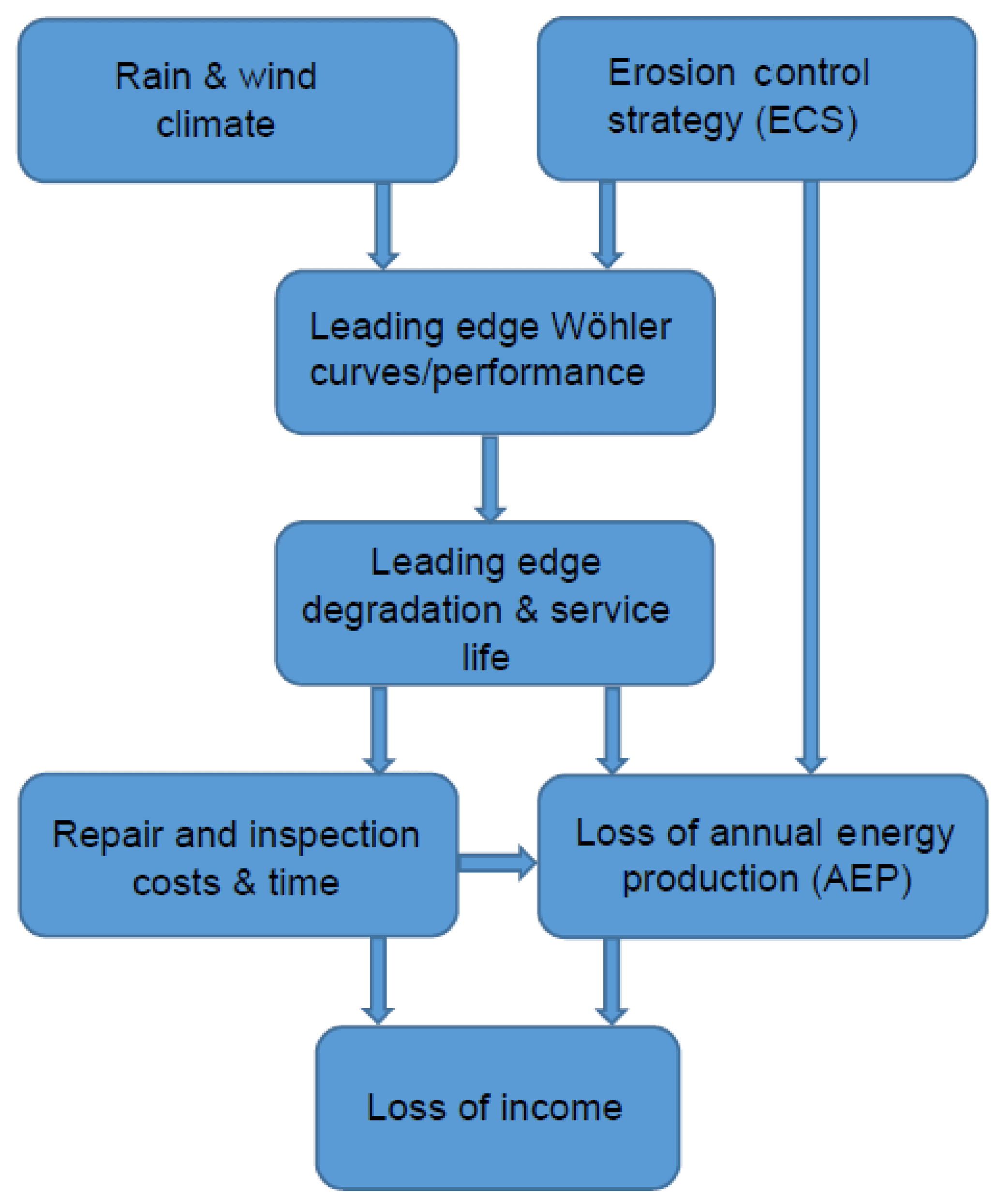
Figure 16Illustration of the framework for calculating the loss of income due to leading-edge erosion.
Figure 16 illustrates in a simplified manner the framework developed here as a tool for selecting the ECS for minimizing the loss of income due to leading-edge erosion, The site-specific rain and wind statistics, the operational data, and ECS determine the erosive loads on the leading edge. Together with the rain erosion test Wöhler curves, these loads are used as input to the cumulative damage rule (Palmgren and Miner) to compute the expected service life. The aerodynamic degradation, the intervals for inspection and repair, and the loss of production due to occasional tip speed reduction are then used to minimize the loss of income. In field operation, precipitation sensors give input to the control system of the turbines to apply the ECS and adapt the control to present weather conditions.
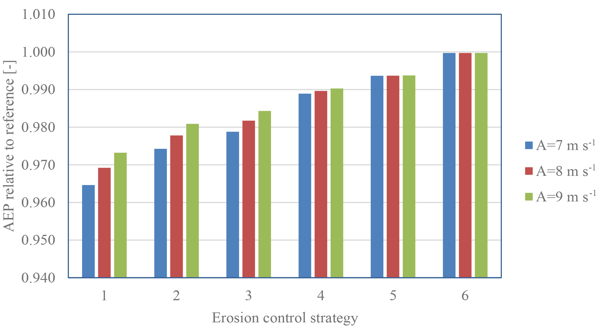
In Fig. 17 the AEP including standstill due to inspection and repair is reflected. It is seen that applying Control Strategy 1, where there is no reduction in the maximum tip speed, the loss of AEP is significant with up to 3.5 % compared to the reference case with no erosion and no inspections and repairs. The loss of AEP is clearly dependent on the wind climate. For low wind speed sites with A=7 m s−1, the loss is greater than for sites with higher wind speeds (A=9 m s−1).
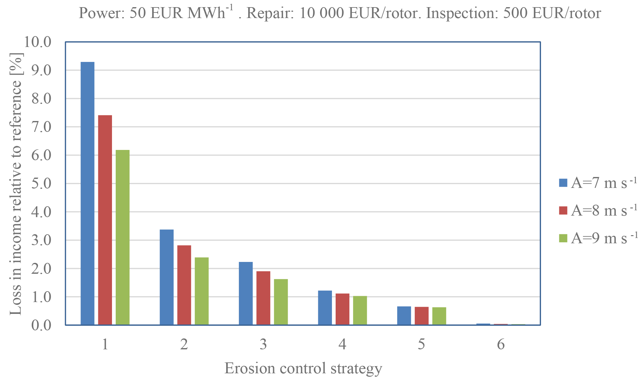
Figure 18Loss of income due to erosion, inspection and repair. Energy: 50 EUR MWh−1. Repair: 10 000 EUR rotor−1. Inspection: 500 EUR rotor−1.
In Figs. 18 to 21, the loss of income due to lost AEP, inspection and repair is seen with the assumption of different costs of energy, inspection and repair. In the plots, the loss of income is significantly simplified and is computed as
where TEP is the total energy production (kWh), EC is the energy cost (EUR MWh−1), NOR is the number of rotor repairs during the life of the turbine, CR is the cost of the repair (EUR rotor−1), NOI is the number of rotor inspections and CI is the cost of each inspection (EUR rotor−1). From the plots it is seen that the loss of income can be significant. The income is very dependent on the energy price and the cost of repair, but a clear trend is that the erosion-safe mode increases the income. Even the very advanced erosion-safe mode – Control Strategy 5, with rather low tip speeds – results in a significant improvement. As an example, Control Strategy 2 can be investigated. Here, the tip speed is reduced from 90 to 70 m s−1 during 5.4 h yr−1 and from 90 to 80 m s−1 during 26.4 h yr−1 due to heavy precipitation. In this case AEP is increased with around 1 % and the income loss is decreased from 15.4 % to 4.5 % in the worst case and from 4.7 % to 2.7 % in the best case, depending on assumptions in cost and wind climate.
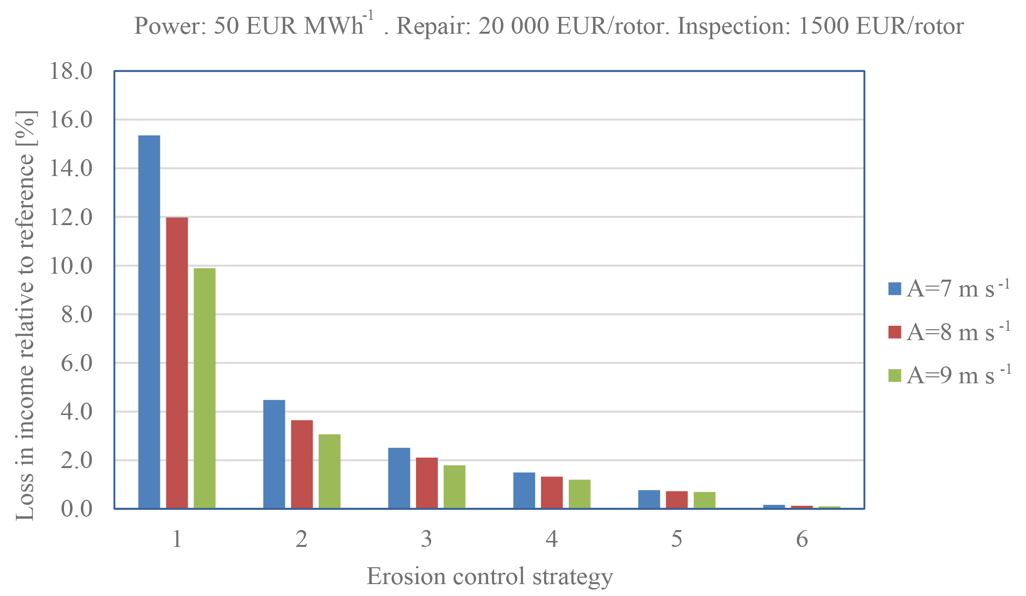
Figure 19Loss of income due to erosion, inspection and repair. Energy: 50 EUR MWh−1. Repair: 20 000 EUR rotor−1. Inspection: 1500EUR rotor−1.
This paper is a concept paper proposing a framework for prediction and mitigation of leading-edge erosion. In order to demonstrate the concept quantitatively, a number of simplifying assumptions and approximations were made.

Figure 20Loss of income due to erosion, inspection and repair. Energy: 250 EUR MWh−1. Repair: 10 000 EUR rotor−1. Inspection: 500 EUR rotor−1.
The assumption of homogenous droplet size for a given rain intensity is obviously an idealization of reality. For a given rain event the droplets sizes are distributed as explained in Sect. 4. These correlations may vary a lot between different types of precipitation, climates, temperatures, levels of pollution, etc. Still the median droplet size and the frequency of large droplets generally increase with increasing rain intensity.
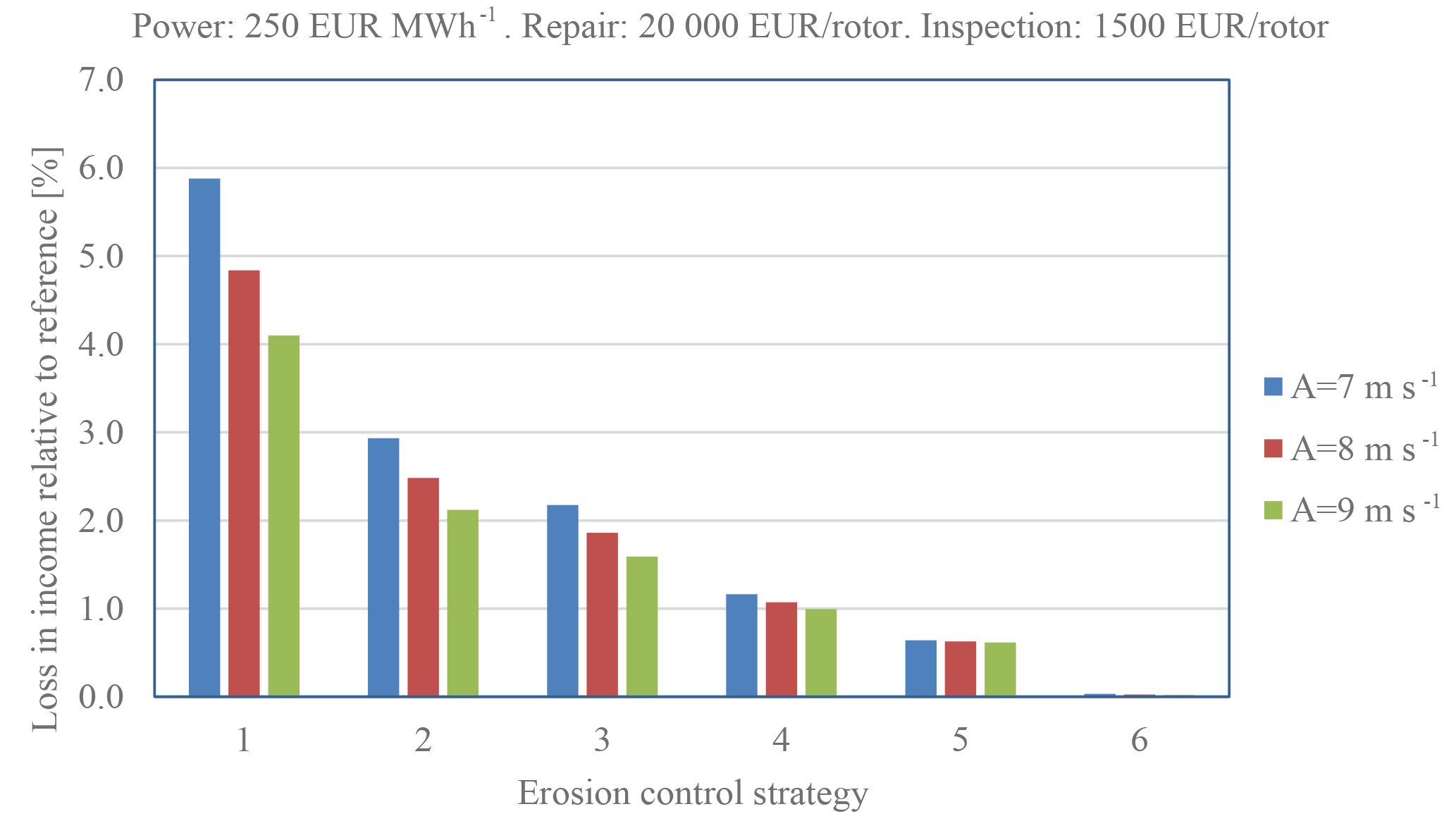
Figure 21Loss of income due to erosion, inspection and repair. Energy: 250 EUR MWh−1. Repair: 20 000 EUR rotor−1. Inspection: 1500 EUR rotor−1.
The assumption that the damage increment scales with the kinetic energy and that the Wöhler curve for one droplet size can be extrapolated to other droplet sizes as suggested in Sect. 3.2 may be controversial. However, there must be a strong correlation between the droplet diameter and the incremental damage. Very small droplets affect only the material very close to the surface. For surface cracking of brittle top coats, the many impacts with smaller droplets may generate more accumulated damage than the few large droplets as demonstrated by Amirzadeh et al. (2017b). For damage modes related to body waves propagating into the structure, affecting the material below the surface (like delamination and cracks in matrix, filler and top coats), only larger droplets and hail have sufficient kinetic energy and size of stress field to affect the structure below the surface. Thus, the correlation between droplet size and damage increment depends a lot on the material, leading-edge configuration and failure mode.
The assumption that the aerodynamic performance decreases linearly with time is not necessarily true. Typically, there will be a long incubation period, where the surface roughness is nearly unaffected, and then the roughness increases at a high rate.
The correlation between leading-edge damage and loss of aerodynamic performance is not fully understood. The loss depends a lot on the aerodynamic profile of the blade and other factors. However, simulations and wind tunnel tests have been carried out, where leading-edge roughness has been investigated and quantified. The transfer function between lifetime and aerodynamic performance is not understood.
The costs for inspection and repair also vary substantially. They are, however, reported to be significant in recent years, in particular for offshore turbines.
The erosion issue has become significant, as the tip speed has increased along with the development towards larger turbines. Many modern turbines have tip speeds of the order of 80 to 90 m s−1. In order to reduce the shaft torque in future designs, it may be attractive to increase tips speeds even beyond 100 m s−1. Then occasional tip speed reduction for erosion control will be even more important, even when stronger leading-edge designs are developed.
The expenses for establishing erosion control are not assessed. These will relate to control algorithms on the turbine control software, precipitation sensors in each wind turbine park, and connections between the sensor and each turbine.
As demonstrated in Sect. 5.2, the economic potential of erosion-safe mode turbine control is significant. Even if the correlations between precipitation intensity and incremental damage or between degree of erosion and aerodynamic performance are not as strong as assumed here, the cost–benefit balance may still be in favour of erosion control.
A framework for prediction and a mitigation strategy for leading-edge erosion was presented. The model takes into account the entire value chain: leading-edge test data, actual on-site precipitation, erosion rate, loss of production due to erosion, operation and maintenance. The lost energy production due to occasional tip speed reduction is marginal in proportion to the alternative of lost production due to eroded blades. Thus, the cost–benefit balance of erosion control looks very promising and shows great potential for reducing the loss of produced energy due to erosion and the cost of operation and maintenance. To accomplish erosion control there is a need for more knowledge on the correlation between precipitation and erosion for different leading-edge structures and materials and for the development of methods and equipment for on-site nowcasting of precipitation.
Existing data have been analysed, and new data have been generated using models of fatigue behaviour of the material and performance of the wind turbine. The data can be provided by contacting the corresponding author.
| AEP | annual energy production |
| BEM | blade element momentum |
| AOA | angle of attack (rad) |
| CI | cost of inspection per rotor (EUR) |
| CR | cost of repair per rotor (EUR) |
| DTV | damage threshold velocity (m s−1) |
| EC | energy cost (EUR kWh−1) |
| ECS | erosion control strategy |
| ESDAC | European Soil Data Centre |
| GFRP | glass-fibre-reinforced polymer |
| LE | leading edge |
| LEE | leading-edge erosion |
| LEP | leading-edge protection |
| LER | leading-edge roughness (m) |
| NOI | number of inspections per rotor (–) |
| NOR | number of repairs per rotor (–) |
| RET | rain erosion test |
| rpm | revolutions per minute |
| RUSLE | Revised Universal Soil Loss Equation |
| TEP | total energy production (kWh) |
| TRRM | Tropical Rainfall Microwave Mission |
| WA-RET | whirling arm rain erosion tester |
| A | Weibull scale parameter (m s−1) |
| C | Weibull shape parameter (–) |
| c | constant (–) |
| cc | airfoil chord length (m) |
| cdrag | drag coefficient (–) |
| clift | lift coefficient (–) |
| cl | speed of sound in liquid (m s−1) |
| cs | speed of Rayleigh wave in target material (m s−1) |
| D | droplet diameter (m) |
| E0 | 1 J |
| Ek | kinetic energy, of each impact of droplet (J) |
| F | specific impact frequency – impacts per area per time (s−1 m−2) |
| Ir | rain intensity (m s−1) |
| m | exponent of Wöhler curve (–) |
| md | mass (kg) |
| M | Miner sum (–) |
| N | number of droplets per volume (m−3) |
| NEi | number of impacts per unit area to removal of coating (m−2) |
| Ni | number of cycles to fatigue failure (–) |
| ni | number of cycles (–) |
| P0 | rated mechanical power with original control (W) |
| P1 | rated mechanical power with erosion control (W) |
| Q0 | original rated main shaft torque (Nm) |
| t | airfoil thickness (m) |
| ti | test time to removal of coating (s) |
| V | relative volume of water in rain field (–) |
| v | impact velocity (m s−1) |
| vr | droplet falling velocity (m s−1) |
| ρl | specific density of liquid (kg m−3) |
| ρs | specific density of solid (kg m−3) |
| ω0 | maximum rotational speed with original control (rad s−1) |
| ω1 | maximum rotational speed with erosion control (rad s−1) |
JIB had the lead on paper writing, test data analysis and lifetime prediction. CBH contributed mainly on precipitation and CB mainly on wind turbine control, aerodynamics and economy. All contributed to writing the paper.
The authors declare that they have no conflict of interest.
The financial support from Innovation Fund Denmark (6154-00018B) for the
project EROSION (http://www.rain-erosion.dk; last access: 11 September
2018) is gratefully acknowledged. The authors want to acknowledge
PolyTech A/S for kindly providing the laboratory test specimen images.
Permission to use the GPCP annual mean precipitation (Fig. 9) is kindly
granted by Todd Mitchell.
Edited by: Lars
Pilgaard Mikkelsen
Reviewed by: Iham Zidane and one anonymous
referee
Adler, W. F.: Waterdrop Impact Modeling, Wear, 186–187, 341–51, 1995.
Adler, W. F.: Rain impact retrospective and vision for the future, Wear, 233–235, 25–38, 1999.
Amirzadeh, B., Louhghalam, A., Raessi, M., and Tootkaboni, M.: A computational framework for the analysis of rain-induced erosion in wind turbine blades, part I: Stochastic rain texture model and drop impact simulations, J. Wind Eng. Ind. Aerod., 163, 44–54, https://doi.org/10.1016/j.jweia.2016.12.007, 2017a.
Amirzadeh, B., Louhghalam, A., Raessi, M., and Tootkaboni, M.: A computational framework for the analysis of rain-induced erosion in wind turbine blades, part II: Drop impact-induced stresses and blade coating fatigue life, J. Wind Eng. Ind. Aerod., 163, 33–43, https://doi.org/10.1016/j.jweia.2016.12.006, 2017b.
ASTM: ASTM G73-10 – Standard Test Method for Liquid Impingement Erosion Using Rotating Apparatus, Astm, 1–19, https://doi.org/10.1520/G0073-10R17, 2017
Bak, C., Johansen, J., and Andersen, P. B.: Three-Dimensional Corrections of Airfoil Characteristics Based on Pressure Distributions. Proc. the European Wind Energy Conference & Exhibition (EWEC), 27 February–2 March 2006, Athens, Greece, 2006.
Best, A. C.: The size of distribution of raindrops, Q. J. Roy. Meteor. Soc., 76, 16–36, 1950.
Blowers, R. M.: On the Response of an Elastic Solid to Droplet Impact, IMA J. Appl. Mathemat., 5, 167–93, 1969.
Bossanyi, E. A.: Wind Turbine Control for Load Reduction, Vol. 6, Special Review Issue on Advances in Wind Energy, July/September 2003.
Bossanyi, E. A.: GH-Bladed User Manual, Issue 14, Garrad Hassan and Partners Limited, Bristol, UK, 2004.
Bowden, F. P. B. and Brunton, J. H.: The Deformation of Solids by Liquid Impact at Supersonic Speeds, P. R. Soc. A, 263, 433–50, 1961.
Bowden, F. P. B. and Field, J. E.: The Brittle Fracture of Solids by Liquid Impact, by Solid Impact, and by Shock, P. R. Soc. A, 282, 331–52, 1964.
Bringi, V. N., Chandrasekar, V., Hubbert, J., Gorgucci, E., Randeu, W. L., and Schoenhuber, M.: Raindrop size distribution in different climatic regimes from disdrometer and dual-polarized radar analysis, J. Atmos. Sci., 60, 354–365, 2003.
Brøndsted, P., Andersen, S. I., and Lilholt, H.: Fatigue damage accumulation and lifetime prediction of GFRP materials under block loading and stochastic loading, Proceedings, Polymer composites, Expanding the limits, 18th Risø Int. symposium, 1997.
Climate-Charts.com: Climate Charts, available at: http://www.climate-charts.com/World-Climate-Maps.html#rain, last access: December 2017.
Cortés, E., Sánchez, F., O'Carroll, A. Madramany, B., Hardiman, M., and Young, T. M.: On the Material Characterisation of Wind Turbine Blade Coatings: The Effect of Interphase Coating-Laminate Adhesion on Rain Erosion Performance, Materials, 10, 1–22, https://doi.org/10.3390/ma10101146, 2017.
Dear, J. P. and Field, J. E.: High-Speed Photography of Surface Geometry Effects in Liquid/solid Impact, J. Appl. Phys., 63, 1015–1650, 1988.
de Haller, P.: Untersuchungen Über Die Durch Kavitation Hervorgerufenen Korrosionen, Schweizerische Bauzeitung, 243, 243–264, 1933.
DNVGL: RP-0171, Recommended Practice, Testing of rotor blade erosion protection systems, http://www.dnvgl.com, last access: 11 September 2018.
Drela, M.: XFOIL, An Analysis and Design System for Low Reynolds Number Airfoils, Low Reynolds Number Aerodynamics, vol. 54, Springer, Verlag Lec. Notes, 1989.
Eisenberg, D., Laustsen, S., and Stege, J.: Leading Edge Protection Lifetime Prediction Model Creation and Validation, poster presented at the Wind Europe summit 27–29 September 2016, Hamburg, https://windeurope.org/summit2016/conference/allposters/PO078g.pdf (last access: 11 September 2018), 2016.
Evans, A. G., Ito, Y. M., and Rosenblatt, M.: Impact damage thresholds in brittle materials impacted by water drops, J. Appl. Phys., 51, 2473–2482, https://doi.org/10.1063/1.328021, 1980.
Fakhari, A. and Rahimian, M. H.: Simulation of Falling Droplet by the Lattice Boltzmann Method, Commun. Nonlinear Sci., 14, 3046–55, 2009.
FMI: Finnish Meteorological Institute, available at: https://finland.fi/life-society/finlands-weather-and-light/, last access: December 2017.
Foote, G. B. and Toit P.S.: Terminal Velocity of Raindrops Aloft, J. Appl. Meteorol., 8, 249–359, 1969.
Fraisse, A., Bech, J. I., Borum, K. K., Fedorov, V., Johansen, N. F.-J., McGugan, M., Mishnaevsky, L., and Kusano, Y.: Impact fatigue damage of coated glass fibre reinforced polymer laminate, Renew. Energ., 126, 1102–1112, 2018.
Frich, P., Rosenørn, S., Madsen, H., and Jensen, J. J.: Observed precipitation in Denmark 1961–1990, Danish Meteorological Institute, Technical Report 97-8, Copenhagen, Denmark.
Fuglsang, P. and Thomsen, K.: Site-specific design optimization of 1.5-2.0 MW wind turbines, J. Sol. Energ. Eng., 123 , 296–303, 2001.
Gohardani, O.: Impact of erosion testing aspects on current and future flight conditions, Prog. Aerosp. Sci., 47, 280–303, https://doi.org/10.1016/j.paerosci.2011.04.001, 2011.
Gorgucci, E., Baldini, L., and Chandrasekar, V.: What Is the Shape of a Raindrop? An Answer from Radar Measurements, J. Atmos. Sci., 63, 3033–44, 2006.
GPCC: Global Precipitation Climate Centre, available at: http://www.gtn-h.info/about/the-network/gpcc/, last access: December 2017.
GPCP: Global Precipitation Climatology Project, https://www.ncdc.noaa.gov/wdcmet/data-access-search-viewer-tools/global-precipitation-climatology-project-gpcp-clearinghouse, last access: 11 September 2018.
Heymann, F. J.: High-Speed Impact between a Liquid Drop and a Solid Surface, J. Appl. Phys., 40, 5113–5124, 1969.
Hong, Y. L., Din, J., and Jong, S. L.: Statistical and Physical Descriptions of Raindrop Size Distributions in Equatorial Malaysia from Disdrometer Observations, Adv. Meteorol., 2015, 253730, https://doi.org/10.1155/2015/253730, 2015.
Jones, D. M. A. and Sims, A. L.: Climatology of instantaneous rainfall rates, J. Appl. Meteorol., 17, 1135–1140, https://doi.org/10.1175/1520-0450(1978)017<1135:COIRR>2.0.CO;2, 1978.
Jonkman, J. M. and Buhl Jr., M. L.: FAST User's Guide, NREL/EL-500-29798, Golden, CO, National Renewable Energy Laboratory, 2005.
Keegan, M. H., Nash, D. H., and Stack, M. M.: Modelling rain drop impact on offshore wind turbine blades, Proceedings of the TURBO EXPO 2012, 6, 887–898, https://doi.org/10.1115/GT2012-69175, 2012.
Keegan, M. H., Nash, D. H., and Stack, M. M.: On erosion issues associated with the leading edge of wind turbine blades, J. Phys. D., 46, 383001, https://doi.org/10.1088/0022-3727/46/38/383001/meta, 2013.
Kubilay, A., Derome, D., Blocken, B., and Carmeliet, J.: CFD simulation and validation of wind-driven rain on a building facade with an Eulerian multiphase model, Build. Environ., 61, 69–81, https://doi.org/10.1016/j.buildenv.2012.12.005, 2013.
Larsen, T. J., Madsen, H. A., Hansen, A. M., and Thomsen, K.: Investigations of stability effects of an offshore wind turbine using the new aeroelastic code HAWC2, Proceedings of the conference ”Copenhagen Offshore Wind 2005”, 2005.
Liersch, J. and Michael, J.: Investigation of the Impact of Rain and Particle Erosion on Rotor Blade Aerodynamics with an Erosion Test Facility to Enhancing the Rotor Blade Performance and Durability, J. Phys. Conf Ser., 524, 12023, https://doi.org/10.1088/1742-6596/524/1/012023, 2014.
Lindenburg, C. and Schepers, J. G.: Phatas-IV Aero-elastic Modelling, Release, “DEC-1999” and “NOV-2000”, ECN-CX–00-027, 2000.
Macdonald, H., Infield, D., Nash, D. H., and Stack, M. M.: Mapping hail meteorological observations for prediction of erosion in wind turbines, Wind Energ., 19, 777–784, https://doi.org/10.1002/we.1854, 2016.
Mason, B. J. and Andrews, J. B.: Drop-size distributions from vaiours types of rain, Q. J. Roy. Meteor. Soc., 86, 346–353, https://doi.org/10.1002/qj.49708636906, 1960.
Met Office: Met Office, available at: http://www.metoffice.gov.uk/learning/rain/how-much-does-it-rain-in-the-uk, last access: December 2017.
Met.no: Norwegian Meteorological Institute, available at: https://www.google.dk/search?q=annual+rainfall+norway&source=lnms&tbm=isch&sa=X&ved=0ahUKEwiI24Gr7PfUAhXlO5oKHft0AYAQ_AUIBigB&biw=1280&bih=610&dpr=1.5#imgrc=HaVIEUIAJXgzzM:&spf=1499453733523, last access: 11 September 2018.
Miner, M.: Cumulative Damage in Fatigue, J. Appl. Mech, 12, A159–A164, 1945.
Naipal, V., Reick, C., Pongratz, J., and Van Oost, K.: Improving the global applicability of the RUSLE model – adjustment of the topographical and rainfall erosivity factors, Geosci. Model Dev., 8, 2893–2913, https://doi.org/10.5194/gmd-8-2893-2015, 2015.
NASA: NASA, https://www.nasa.gov/, last access: 11 September 2018.
Njiri, J. G. and Söffker, D.: State-of-the-art in wind turbine control: Trends and challenges, Renew. Sustain. Energ. Rev., 60, 377–393, 2016.
OffshoreWindBiz: Siemens Gamesa Starts Repairing Anholt Blades, London Array Up Next, available at: https://www.offshorewind.biz/2018/04/26/, last access: June 2018.
Øye, S.: FLEX 4 – Simulation of Wind Turbine Dynamics. Proceedings of the 28th IEA Meeting of Experts “State of the Art of Aeroelastic Codes for Wind Turbine Calculations”, Technical University of Denmark, Lyngby, Denmark, 71–76, 1996.
Panagos, P., Ballabio, C., Borrelli, P., Meusburger, K., Klik, A., Rousseva, S., Tadic, M.P., Michaelides, S., Hrabalikova, M., Olsen, P., Aalto, J., Lakatos, M., Rymszewicz, A., Dumitrescu, A., BeguerÃa, S., and Alewell, C.: Rainfall erosivity in Europe, Sci. Total Environ., 511, 801–814, https://doi.org/10.1016/j.scitotenv.2015.01.008, 2015.
Panagos, P., Borrelli, P., Meusburger, K., Yu, B., Klik, A., Lim, K. J, Yang, J. A., Ni, J., Miao, C., Chattopadhyay,N., Sadeghi, S. H., Hazbavi, Z., Zabihi, M., Larionov, G. A., Krasnov, S. F., Gorobets, A. V., Levi, Y., Erpul, G., Birkel, C., Hoyos, N., Naipal, V., Oliveira, P. T. S., Bonilla, C.A., Meddi, M., Nel, W., Dashti, H. A., Boni, M., Diodato, N., Van Oost, K., Nearing, M., and Ballabio, C.: Global rainfall erosivity assessment, based on high-temporal resolution rainfall records, Sci. Rep., 7, 4175, https://doi.org/10.1038/s41598-017-04282-8, 2017.
Peel, M. C., Finlayson, B. L., and McMahon, T. A.: Updated world map of the Köppen-Geiger climate classification, Hydrology and Earth System Sciences Discussions, European Geosciences Union, 11, 1633–1644, https://doi.org/10.5194/hess-11-1633-2007, 2007.
Poulsen, T., Hasager, C. B., Jensen, and C. M: The Role of Logistics in Practical Levelized Cost of Energy Reduction Implementation and Government Sponsored Cost Reduction Studies: Day and Night in Offshore Wind Operations and Maintenance Logistics, Energies, 10, 1–28, https://doi.org/10.3390/en10040464, 2017.
Prayogo, G., Homma, H., Soemardi, T. P., and Danadorno, A. S.: Impact Fatigue Damage of GFRP Materials Due to Repeated Raindrop Collisions, Trans. Indian Inst. Met., 64, 501–506, https://doi.org/10.1007/s12666-011-0078-5, 2011.
Renews: Renews, available at: http://renews.biz/110279/anholt-grapples-with-blade-fix/, last access: 11 September 2018a.
Renews: Renews, available at: http://renews.biz/110465/london-array-braced-for-blade-fix/, last access: 11 September 2018b.
Ronold, K. and Echtermeyer, A.: Estimation composite of fatigue laminates curves for design of composite laminates, Compos, Part A, Appl. Sci. Manuf., 27, 485–491, https://doi.org/10.1016/1359-835X(95)00068-D, 1996.
Sareen, A., Sapre, C. A., and Selig, M. S.: Effects of leading edge erosion on wind turbine blade performance, Wind Energy, 17, 1531–1542, 2014.
Siddons, C., Stack, M. M., and Nash, D. H.: An experimental approach to analysing rain droplet impingement on wind turbine blade materials, presented at EWEA Annual Conference and Exhibition 2015.
Slot, H. M., Gelinck, E. R. M., Rentrop, C., and van der Heide, E.: Leading edge erosion of coated wind turbine blades: Review of coating life models, Renew. Energ., 80, 737–848, https://doi.org/10.1016/j.renene.2015.02.036, 2015.
SMHI: SMHI Swedish Meteorology and Hydrology Institute, available at: http://www-markinfo.slu.se/eng/climate/ned.html, last access: December 2017.
Smith, J. A., Hui, E., Steiner, M., Baeck, M. L., Krajewski, W. F., and Ntelekos, A. A.: Variability of rainfall rate and raindrop size distributions in heavy rain, Water Resour. Res., 45, 1–12, https://doi.org/10.1029/2008WR006840, 2009.
Springer, G., Yang, C., and Larsen, P.: Analysis of Rain Erosion of Coated Materials, J. Compos. Mater., 8, 229–252, 1974.
Springer, G., Yang, C., and Larsen, P.: Model for the rain erosion of fiber reinforced composites, AIAA J., 13, 877–883, 1975.
Stephenson, S.: Wind blade repair: Panning, safety, flexibility, Composites World, 2011.
Wittrup, S.: Dong og Siemens giver Horns Rev 2 storstilet vinge-makeover, Ingeniøren, 2015 (in Danish).
Wobben, A.: Patent US2003/0165379, available at: https://www.google.com/patents/US20030165379 (last access: 11 September 2018), 2003.
Woods, R. D.: Screening of Surface Wave in Soils, Journal of the Soil Mechanics and Foundations Division, 94, 951–980, 1968.
World Atlas: World Atlas, available at: http://www.worldatlas.com/articles/the-ten-wettest-places-in-the-world.html, last access: December 2017.
WorldClim: WorldClim, available at: https://dasgeographer.wordpress.com/2013/09/05/world-precipitation-patterns/, last access: December 2017.
Zidane, I. F., Saqr, K. M., Swadener, G., Ma, X., and Shehadeh, M. F.: On the role of surface roughness in the aerodynamic performance and energy conversion of horizontal wind turbine blades: a review, Int. J. Energy Res., 40, 2054–2077, https://doi.org/10.1002/er.3580, 2016.
Zidane, I. F., Saqr, K., M., Swadener, G., Ma, X., and Shehadeh, M. F.: Computational Fluid Dynamics Study of Dusty Air Flow over NACA 63415 Airfoil for Wind Turbine, Jurnal Teknologi, 70, 1–6, 2017.