the Creative Commons Attribution 4.0 License.
the Creative Commons Attribution 4.0 License.
 | 24 Oct 2018
Online model calibration for a simplified LES model in pursuit of real-time closed-loop wind farm control
Bart M. Doekemeijer
Sjoerd Boersma
Lucy Y. Pao
Torben Knudsen
Jan-Willem van Wingerden
Wind farm control often relies on computationally inexpensive surrogate models to predict the dynamics inside a farm. However, the reliability of these models over the spectrum of wind farm operation remains questionable due to the many uncertainties in the atmospheric conditions and tough-to-model dynamics at a range of spatial and temporal scales relevant for control. A closed-loop control framework is proposed in which a simplified model is calibrated and used for optimization in real time. This paper presents a joint state-parameter estimation solution with an ensemble Kalman filter at its core, which calibrates the surrogate model to the actual atmospheric conditions. The estimator is tested in high-fidelity simulations of a nine-turbine wind farm. Exclusively using measurements of each turbine's generated power, the adaptability to modeling errors and mismatches in atmospheric conditions is shown. Convergence is reached within 400 s of operation, after which the estimation error in flow fields is negligible. At a low computational cost of 1.2 s on an 8-core CPU, this algorithm shows comparable accuracy to the state of the art from the literature while being approximately 2 orders of magnitude faster.
- Article
(14070 KB) - Full-text XML
- BibTeX
- EndNote


Over the past decades, global awakening on climate change and the environmental, political and financial issues concerning fossil fuels have been catalysts for the growth of the renewable energy industry. As the primary energy demand in Europe is projected to decrease by 200 million tonnes of oil equivalent from 2016 to 2040, there is an additional shift in the energy source used to meet this demand (International Energy Agency, 2017). Shortly after 2030, onshore and offshore wind energy are projected to become the main source of electricity for the European Union. By then, about 80 % of all new capacity added is projected to come from renewable energy sources, enabled by a favorable political climate.
While these developments have clear benefits, an important problem with wind energy is that the rotational speed of most commercial turbines is decoupled from the electricity grid frequency via each turbine's power electronics (Aho et al., 2012). As the current grid-connected fossil fuel plants are replaced by non-synchronous renewable energy plants, the inertia of the electricity grid will decrease, making it less stable and more prone to machine damage and blackouts (Ela et al., 2014). Therefore, there is a strong need for wind farms and other renewable sources to provide ancillary grid services. Wind farm control aimed at increasing the grid stability is more commonly defined as active power control (APC). In APC, the power production of a wind farm is regulated to meet the power demand of the electricity grid, which may change from second to second.
Existing literature on wind farm control has mainly focused on maximizing the power capture (e.g., Rotea, 2014; Gebraad and van Wingerden, 2015; Gebraad et al., 2016; Munters and Meyers, 2017). However, literature on APC has been receiving an increasing amount of attention (e.g., Fleming et al., 2016; Van Wingerden et al., 2017; Boersma et al., 2017). The main challenges in wind farm control are the large time delays caused by the formation of wakes, the many uncertainties in the atmospheric conditions, and the questionable reliability of surrogate models over the wide spectrum of wind farm operation. (See Boersma et al. (2017) and Knudsen et al. (2015) for state-of-the-art overviews of control and control-oriented modeling for wind farms.) While there has been success with model-free methods for power maximization (Rotea, 2014), it is unclear to what degree such methods can be used for power forecasting. Furthermore, model-free methods typically have long settling times, making them intractable for APC. On the other hand, for model-based approaches, the aforementioned challenges make it impossible for any model to reliably provide power predictions in an open-loop setting. Hence, a model-based approach in which a surrogate wind farm model is actively adjusted to the present conditions is a necessity for reliable and computationally tractable APC algorithms. This closed-loop wind farm control framework, consisting of three components, is shown in Fig. 1.
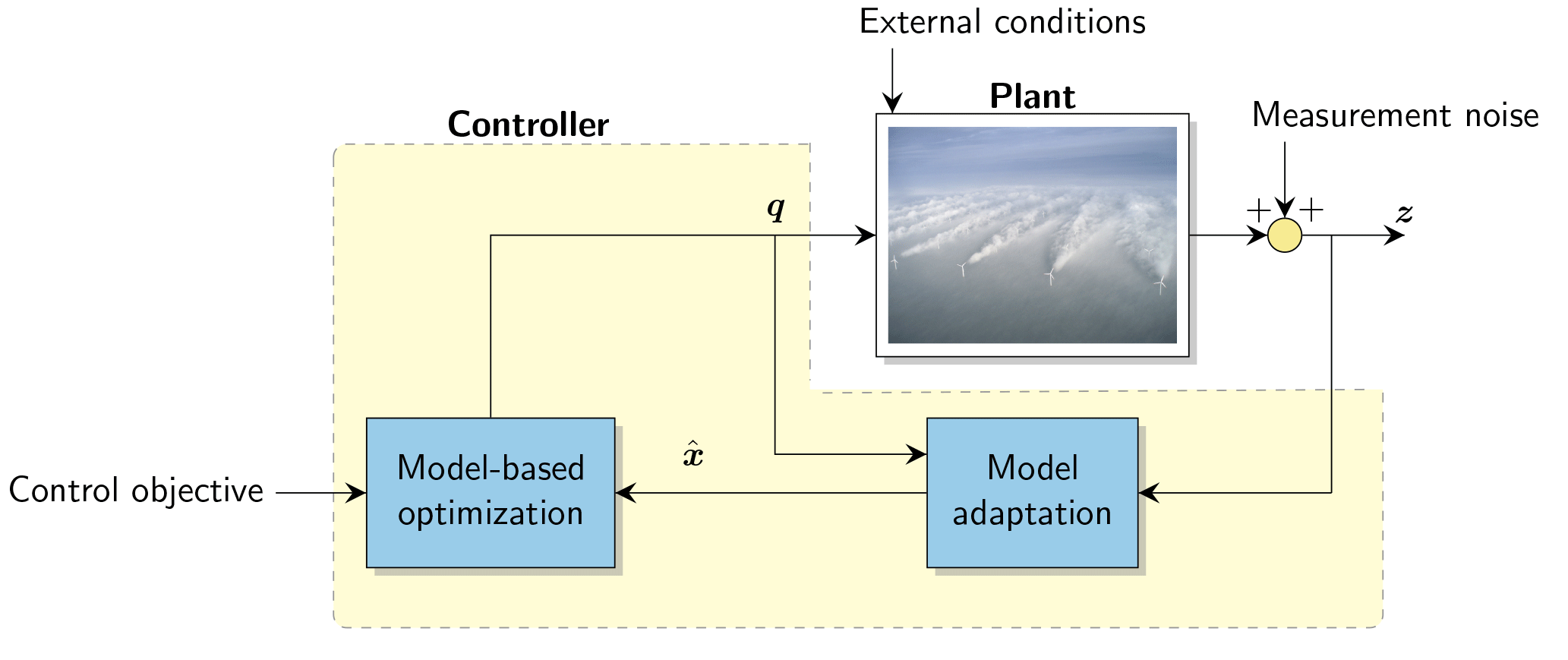
Figure 1Closed-loop wind farm control framework. Measurements z (e.g., SCADA or lidar data) are fed into the controller. First, the state of the surrogate model x is estimated to represent the actual atmospheric and turbine conditions inside the wind farm. Secondly, using the calibrated model, an optimization algorithm determines the control policy (e.g., yaw angles) for all turbines q. This control policy may be a set of constant operating points, but can also be time-varying, depending on whether the surrogate model is time-varying and the employed optimization algorithm. The photograph of the wind farm is from Christian Steiness.
The first component of the closed-loop framework is a computationally inexpensive surrogate model that accurately predicts the power production of the wind farm ahead of time, on a timescale relevant for control. The most commonly used surrogate models in wind farm control are steady-state models, which are heuristic and neglect all temporal dynamics (Boersma et al., 2017). While some of these models have shown success in wind tunnel tests (Schreiber et al., 2017) and field tests (Fleming et al., 2017a, b) for power maximization, the actuation frequency is limited to the minutes timescale, since the flow and turbine dynamics are predicted on the minutes timescale. Furthermore, time-ahead predictions with these models are limited to the steady state, limiting their use for APC. There is a smaller yet significant number of dynamic surrogate wind farm models (Boersma et al., 2018; Munters and Meyers, 2017; Shapiro et al., 2017a) that attempt to include the dominant temporal dynamics inside the farm. These models can be used for control on the seconds timescale, and furthermore allow time-ahead predictions, some even under changing atmospheric conditions. Specifically, the dynamic surrogate model employed in Shapiro et al. (2017a) is computationally feasible, but only models the flow in one dimension and furthermore allows no turbine yaw or changes in the wind direction, limiting its applicability. Furthermore, the dynamical model in Munters and Meyers (2017) has shown success for closed-loop control applications, but it is too computationally expensive for any kind of real-time control, and the authors present their results solely as a benchmark case. In the work presented here, the model described in Boersma et al. (2018) is used, which is a two-dimensional (2-D) large eddy simulation (LES) code with wind farm control as its main objective. This dynamic surrogate model, named “WindFarmSimulator” (WFSim), includes yaw and axial induction actuation, turbine-induced turbulence effects, and spatially and temporally varying inflow profiles, with a moderate computational cost.
The second component of the closed-loop framework is an algorithm that adjusts the surrogate model's parameters to improve its accuracy online using flow and/or turbine measurements (e.g., supervisory control and data acquisition, SCADA, data; lidar measurements; meteorological masts). In terms of control, this turns into a joint estimation problem, in which both the model state and a subset of model parameters are estimated online. Currently, the optimization algorithms presented in Munters and Meyers (2017) and Vali et al. (2017) have assumed full state knowledge, conveniently ignoring the step of model adaptation. Literature on state reconstruction and model calibration for dynamical wind farm models is sparse, limited to linear low-order models and/or common estimation algorithms. Gebraad et al. (2015) designed a traditional Kalman filter (KF) for their low-fidelity model, showing marginal improvements compared to optimization using a static model. Shapiro et al. (2017a) present a one-dimensional dynamic wake model used with receding horizon control for secondary frequency regulation, using an estimation algorithm following Doekemeijer et al. (2016). Furthermore, Iungo et al. (2015) used dynamic mode decomposition to obtain a reduced-order model of the wind farm dynamics, which was then combined with a traditional KF for state estimation. To the best of the authors' knowledge, none of these methods have explored more sophisticated models such as WFSim, and often only use simple state estimation algorithms that are lacking in terms of accuracy and computational tractability.
The third component of the closed-loop framework is an optimization algorithm, which typically is a gradient-based or nonlinear optimization algorithm (Gebraad et al., 2016) for steady-state models, and a predictive optimization method for dynamical models (Goit and Meyers, 2015; Siniscalchi-Minna et al., 2018; Vali et al., 2017). A more in-depth discussion on optimization algorithms is out of the scope of this article.
The focus of this work is on a model adaptation algorithm for WFSim, which balances estimation accuracy and computational complexity. In previous work (Doekemeijer et al., 2016, 2017), state estimation using flow measurements downstream of each turbine has shown success using an ensemble KF (EnKF), with a computational cost several orders of magnitude lower than traditional KF methods. The main contributions of this article specifically are
-
the additional adaptation to a mismatch in atmospheric conditions (specifically the ambient wind speed and turbulence intensity),
-
the option to use turbine's power signals in addition to, or instead of, flow measurements,
-
a further reduction in the computational complexity,
-
and a comparison of the EnKF with the state of the art in the literature.
The structure of this article is as follows. In Sect. 2, the surrogate model will be introduced. In Sect. 3, a time-efficient, online model calibration algorithm for dynamical wind farm models is detailed. This calibration algorithm is validated and compared with standard algorithms in the literature in high-fidelity simulations in Sect. 4. The article is concluded in Sect. 5.
The framework of Fig. 1 requires a surrogate model of the wind farm. In this work, that is the WindFarmSimulator (WFSim) model presented by Boersma et al. (2018). This model is particularly suited as it includes both yaw and axial induction actuation and yields a relatively high accuracy with a relatively low computational cost1. The aim of this section is to give a summary of the surrogate model, rather than a full derivation and motivation of the assumptions made. The reader is referred to Boersma et al. (2018) for more information.
Fundamentally, WFSim is based on the 2-D unsteady incompressible Navier–Stokes (NS) equations. The surrogate model can be completely described by the flow and rotor dynamics in a horizontal plane at hub height. WFSim deviates from a traditional 2-D NS model in two ways. Firstly, the diffusion term is neglected, as it plays a negligible role due to the low viscosity of air. Secondly, the dissipation term in the lateral direction in the continuity equation is multiplied by a factor of 2 to approximate flow dissipating in the vertical flow dimension. Other vertical flow contributions such as vertical meandering and shear are neglected. The subgrid-scale model is formulated using an eddy-viscosity assumption in combination with Prandtl's mixing length model. The mixing length is parameterized as a function of the spatial location, increasing linearly with distance from the downstream rotor, starting at zero at distance d′ downstream and peaking at distance d, where ℓs defines the slope of the mixing length. Basically, the larger ℓs, the quicker wakes recover to their free-stream properties. Furthermore, the turbines are modeled using the non-rotating (static) actuator disk model, projected onto the 2-D plane at hub height. The turbine is assumed to be a rigid object applying a 2-D force vector on the flow. Both the turbine forcing term and the turbine power output are scaled by tuning factors cf and cp, respectively, to account for unmodeled effects. Together with the three parameters from the turbulence model, this leads to a total of five tuning parameters.
These NS equations are solved over a spatially and temporally discretized domain (Boersma et al., 2018). Dirichlet boundary conditions for the longitudinal and lateral velocity are applied on one side of the grid for inflow, while Neumann boundary conditions are applied on the remaining sides for the outflow. The surrogate model reduces to a nonlinear discrete-time deterministic state-space model as
where xk∈ℝN is the system state at time k, which is a column vector containing the collocated longitudinal flow velocity at each cell in the domain , the lateral flow velocity at each cell in the domain , and the pressure term at each cell in the domain , with and . The state xk is formulated as
Empirically, good results have been achieved with cell dimensions of about 30–50 m in width and length, resulting in N with a typical value on the order of 103–104 for six- to nine-turbine wind farms (Boersma et al., 2018; Doekemeijer et al., 2016, 2017; Vali et al., 2017). Such a number of states may seem very small for LES simulations, yet is very high for control purposes. Furthermore, qk∈ℝO includes the system inputs, i.e., the turbine control settings: the turbine yaw angles γi and the thrust coefficients for , with NT being the number of turbines. The system outputs zk∈ℝM are defined by sensors. It can include, among others, flow field measurements (zk⊂xk) and power measurements. We define the integer with as the total number of flow field measurements. The nonlinear functions f and h are the state forward propagation and output equation, respectively.
The computational cost may vary from 0.02 s for two-turbine wind farms with states (e.g., in Doekemeijer et al., 2017) to 1.2 s for states for medium-sized wind farms (e.g., in Boersma et al., 2018), for a single time-step forward simulation on a single desktop CPU core. The computational complexity of the model is what motivates the use of time-efficient estimation algorithms in this work, and time-efficient predictive control methods for optimization in related work (Vali et al., 2017). Here, the limits of computational cost are explored to maximize model accuracy while still allowing real-time control. Note that research on the computational feasibility of optimization algorithms using WFSim is ongoing.
Due to the limited accuracy of surrogate wind farm models, and due to the many uncertainties in the environment, surrogate models often yield predictions with significant uncertainty in the wind flow and power capture inside a wind farm. Since control algorithms largely rely on such predictions, this may suppress gains or even lead to losses inside a wind farm. Unfortunately, higher-fidelity models are computationally prohibitively expensive for control applications. Hence, lower-fidelity surrogate models are calibrated online using readily available measurement equipment.
In this section, first the challenges for real-time model calibration for the surrogate “WFSim” model described in Sect. 2 will be highlighted in Sect. 3.1. Secondly, a mathematical framework for recursive model state estimation will be presented in Sect. 3.2. Thirdly, a number of nonlinear state estimation algorithms are presented in Sects. 3.3 to 3.5, building up from the industry standard to the state of the art in the literature. Finally, a robust and computationally efficient model calibration solution is synthesized in Sect. 3.6, which allows for the simultaneous estimation of the boundary conditions, model parameters, and the model states of WFSim in real time using readily available measurements from the wind farm.
Note that we will henceforth refer to the estimation of x as state(-only) estimation. The estimation of both model states and model parameters such as ℓs is referred to as (joint) state-parameter estimation.
3.1 Challenges
Online model calibration for WFSim is challenging for a number of reasons. First of all, the model is nonlinear, and thus the common linear estimation algorithms cannot be used without linearization, which limits accuracy (Boersma et al., 2018). Secondly, an estimation solution relying on WFSim is sensitive to instability when the model state sufficiently deviates from the continuity equation. Finally, the surrogate model typically has on the order of N∼103–104 states, which is extraordinarily high for control applications. However, real-time estimation is a necessity for real-time model-based control, and thus one needs to find a trade-off between accuracy while guaranteeing state updates at a low computational cost.
3.2 General formulation
This section summarizes the basics of the KF, which is the literature standard for state estimation in control. The goal of a KF is to recursively estimate the unmeasured states of a dynamical system through noisy measurements. Assumed here is a system (the wind farm) represented mathematically by a discrete-time stochastic state-space model with additive noise,
where k is the time index, x∈ℝN is the unobserved system state, z∈ℝM are the measured outputs of the system, q∈ℝO and w∈ℝN are the controllable inputs and process noise, respectively, that drive the system dynamics, and v∈ℝM is measurement noise. Furthermore, we assume w and v to be zero-mean white Gaussian noise with covariance matrices
with E the expectation operator. Estimates of the state xk, denoted by , are computed based on measurements from the real system. Here, means an estimate of the state vector x at time k, using all past measurements and inputs 𝓩ℓ as
State estimates are based on the internal model dynamics and the measurements, weighted according to their probability distributions. We aim to find an optimal state estimate, in which optimality is defined as unbiasedness, , and when the variance of any linear combination of state estimation errors (e.g., the trace of ) is minimized.
In reality, the assumed model described by f and h always has mismatches with the true system, and the assumptions in Eq. (3) often do not hold. Further, the matrices Qk, Rk, and Sk are usually not known and are rather considered to be tuning parameters, used to shift the confidence levels between the internal model and the measured values. For R≪Q, estimations will heavily rely on the measurements, while for Q≪R, estimations will mostly rely on the internal model. Kalman filtering remains one of the most common methods of recursive state estimation. KF algorithms typically consist of two steps.
-
A state and output forecast, including their uncertainties (covariances):
In Eqs. (5) and (6), and are the forecasted system state vector and measurement vector, respectively.
-
An analysis update of the state vector, where the measurements are fused with the internal model:
Here, in Eq. (10) is the pseudo-inverse of , since this matrix is not necessarily invertible.
Traditionally, state estimation for linear dynamic models is done using the linear KF (Kalman, 1960). However, this is not a viable option here, as the surrogate model is nonlinear. Rather, a number of nonlinear KF variants are looked upon.
3.3 Extended Kalman filter (ExKF)
Linearization of the surrogate model is the most popular and straight-forward solution to the issue of model nonlinearity, as done in the extended KF (ExKF). The ExKF has shown success in academia and industry (Wan and Van Der Merwe, 2000) and is perhaps the most popular nonlinear KF. However, it has a number of disadvantages. As described in Sect. 3.1, model linearization is troublesome. Furthermore, for surrogate models with many states such as WFSim, the ExKF has an additional challenge: computational complexity. The operation in Eq. (10) includes a matrix inversion with a computational complexity of 𝒪(M3), and the ExKF furthermore includes two matrix multiplications each with a complexity of 𝒪(N3). As there are significantly fewer measurements than states (M≪N) for the problem at hand, these matrix multiplications dominate the computational cost. The ExKF has a CPU time on the order of 101 s for a two-turbine wind farm, which may be too large for our purposes. To reduce computational cost in the ExKF, the surrogate model and/or the covariance matrix P have to be simplified. This is not further explored here. Instead, two KF approaches will be explored that directly use the nonlinear system for forecasting and analysis updates. Doing so, we circumvent the problems with linearization, and additionally better maintain the true covariance of the system state.
3.4 The unscented Kalman filter (UKF)
The unscented Kalman filter (UKF) relies on the so-called “unscented transformation” to estimate the means and covariance matrices described by Eqs. (5) to (9). The conditional state probability distribution of xk knowing 𝓩k is again assumed to be Gaussian. In the UKF, firstly a number of sigma points (also referred to as “particles”) are generated such that their mean is equal to and their covariance is equal to Cov(xk,xk). Secondly, each particle is propagated through the nonlinear system dynamics (f, h). Thirdly, the mean and covariance of the forecasted state probability distribution is again approximated by a weighted mean of these forecasted sigma points (Wan and Van Der Merwe, 2000).
Mathematically, we define the ith particle as , which is a realization of the conditional probability distribution of xk given 𝓩ℓ. The UKF follows a very similar forecast and analysis update approach as the traditional KF in Eqs. (5) to (12), yet applied to a finite set of particles (Wan and Van Der Merwe, 2000).
-
For the forecast step, a particle-based approach is taken.
- i.
A total of particles, with N equal to the state dimension, are (re)sampled to capture the mean and covariance of the conditional state probability distribution by
where is a scaling parameter, α determines the spread of the particles around the mean, and κ is a secondary scaling parameter typically set to 0 (Wan and Van Der Merwe, 2000). The vector is the estimated state vector calculated as , where the weight of each particle's mean and covariance is given by
and β is used to incorporate prior knowledge on the probability distribution. In this work, β=2 is assumed, which is stated to be optimal for Gaussian distributions (Wan and Van Der Merwe, 2000).
- ii.
Each particle is propagated forward in time using the expectation of the nonlinear model as
where is defined as the system output corresponding to the particle .
- iii.
The expected state and expected output are calculated as
and the covariance matrices are (re-)estimated from the forecasted ensemble by
- i.
-
For the analysis step, one can apply the same equations as in Eqs. (10) to (12).
The UKF has been shown to consistently outperform the ExKF in terms of accuracy, since it uses the nonlinear model for forecasting and covariance propagation. However, this does come at an increased computational cost. Namely, particles are required to capture the mean and covariance of the conditional state probability distribution. This implies that 2N+1 function evaluations are required for each UKF update. Even for a two-turbine wind farm in WFSim, a computational cost of 1×10² s per iteration () would not be surprising. While Eq. (14) can easily be parallelized, computational complexity remains troublesome, especially for larger wind farms. The issue of computational complexity is tackled by the ensemble KF.
3.5 The ensemble Kalman filter (EnKF)
The ensemble Kalman filter (EnKF; Evensen, 2003) is very similar to the UKF in that it relies on a finite number of realizations (the “sigma points” or “particles” in the UKF) to approximate the mean and covariance of the conditional probability distribution of xk knowing 𝓩k. However, whereas the UKF relies on a systematic way of distributing the particles such that the mean and covariance of the conditional probability distribution p[xk|𝓩k] are equal to that of the particles, the EnKF relies on random realizations, without guarantees that the mean and covariance are captured accurately. However, the EnKF has been shown to work well in a number of applications, with typically far fewer particles than states, i.e., Y≪N (Gillijns et al., 2006; Houtekamer and Mitchell, 2005). The forecast and update step are very similar to that of the UKF.
-
In the UKF the particles are redistributed at every time step, in contrast to the EnKF. Rather, the EnKF propagates the particles forward without redistribution. We define the ith particle as , which is a realization of the conditional probability distribution p[xk|𝓩ℓ]. The forecast steps are
- i.
Each particle is propagated forward in time using the nonlinear system dynamics, and with the realizations of noise terms w and v denoted by and , generated using MATLABs randn(…) function.
- ii.
The expected state and output are identically calculated as in the UKF using Eq. (15) with . The covariance matrices are (re-)estimated from the forecasted ensemble by
- i.
-
For the analysis step, one applies Eq. (10) to determine the Kalman gain Lk. Then, each particle is updated individually as
Note that, in contrast to the ExKF and the UKF, the state covariance matrix Px (see Eqs. 7 and 12) need not be calculated explicitly in the EnKF. This, in combination with the small number of particles Y≪N, is what makes the EnKF computationally superior to the UKF (and often also computationally superior to the ExKF). However, this reduction in computational complexity comes at a price. The disadvantages of the EnKF are discussed in the next section.
Challenges in the EnKF for small number of particles
The caveat to representing the conditional state probability distribution with fewer particles than states, Y≪N, is the formation of inbreeding and long-range spurious correlations (Petrie, 2008). The former, inbreeding, is defined as a situation where the state error covariance matrix Px is consistently underestimated, leading to state estimates that incorrectly rely more on the internal model. One straight-forward method to address this is called “covariance inflation”, in which Px (or rather, the ensemble from which Px is calculated) is “inflated” to correct for the underestimated state uncertainty (Petrie, 2008). Mathematically, this is achieved by applying
before the analysis step, with r∈ℝ the inflation factor, typically with a value of 1.01–1.25.
The latter problem, long-range spurious correlations, can be better visualized in Fig. 2.
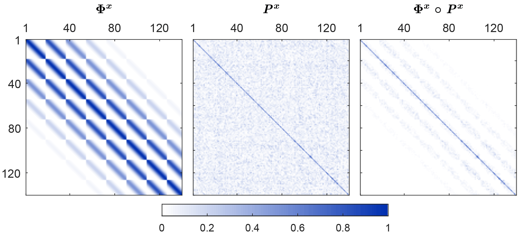
Figure 2Long-range spurious correlations arise in the case where a covariance matrix is described by a small number of particles. Using physical knowledge of the system, these undesired correlations can be corrected. Φx is the localization matrix. Applying localization, the covariance of physically nearby states are multiplied with a value close to 1, and the covariance of physically distant states are multiplied with a value close to 0. In our example case, this results in the localized covariance matrix Φx∘Px, where ∘ is the element-wise product.
In particle-based approaches, the covariance terms cannot be captured exactly. This may lead to the formation of small yet nonzero covariance terms between states and outputs which, in reality, are uncorrelated. This can lead to the drift of unobservable states, and eventually to instability of the KF. Increasing the number of particles is the most straight-forward solution to this problem, but comes at a huge computational cost. A better alternative is “covariance localization”, where physical knowledge of the states and measurements is used to steer the sample-based covariance matrices. Recall that in the surrogate model of Sect. 2, the model states are the velocity and pressure terms inside the wind farm at a physical location. Define that the ith state entry (xk)i belongs to a physical location in the farm si. Then, looking at an arbitrary state covariance term (i,j),
we define the physical distance between these two states as Now, we introduce a weighting factor into our covariance matrices by multiplying physically distant states with a value close to 0, and multiplying physically nearby states with a value close to 1. A popular choice for such a weighting function is Gaspari–Cohn's fifth-order discretization of a Gaussian distribution (Gaspari and Cohn, 1999), given by
with a normalized distance measure, with L the cut-off distance. Applying Eq. (24) for the covariance matrices and we can define the localization matrices
where is the normalized distance between two measurements i and j, and is the normalized distance between state i and measurement j, respectively. Finally, localization and inflation can be incorporated into Eqs. (20) and (21) by
where ∘ is the element-wise product (Hadamard) of the two matrices. The improvement in terms of computational efficiency and estimation performance is displayed in Fig. 3.
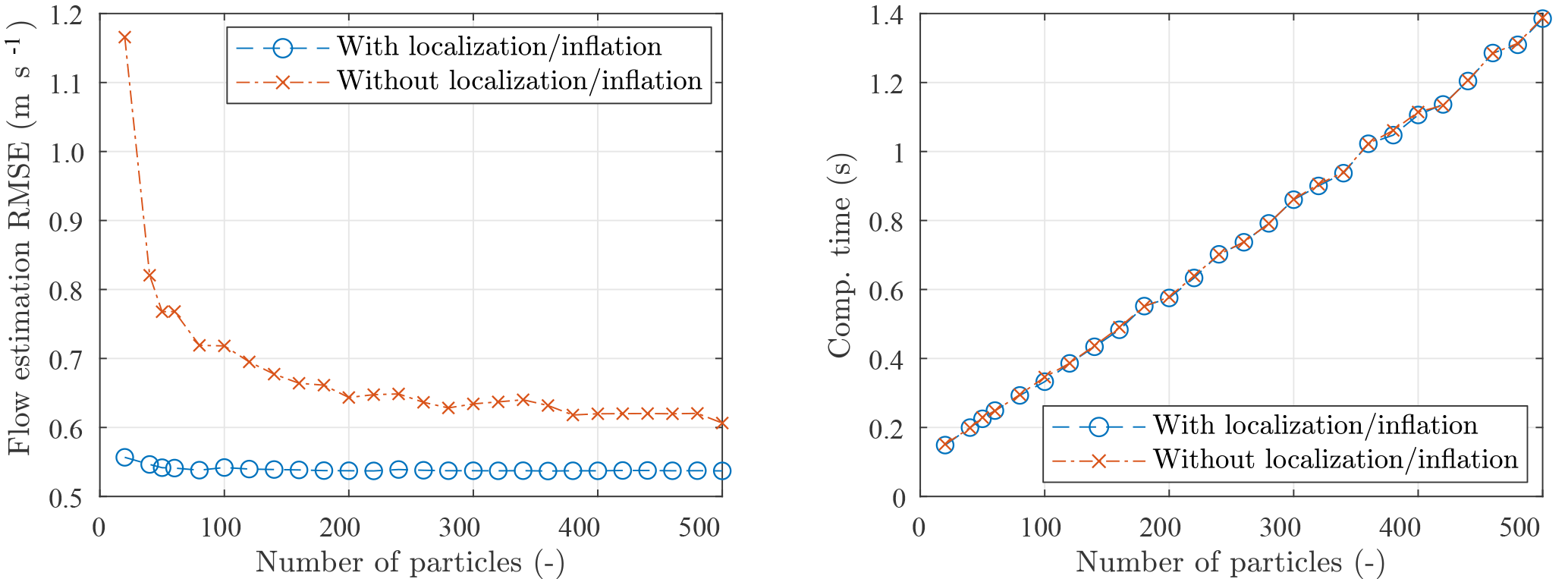
Figure 3This figure shows the estimation performance and computational cost (parallelized, 8 cores) of the EnKF for a range of ensemble sizes, with and without inflation and localization. Great improvement is seen for estimation accuracy, at no additional computational cost. The simulation scenario is described in detail in Sect. 4.2, and the results presented here are rather meant as an indication.
A significant increase in performance is shown, especially for smaller numbers of particles. This is in agreement with what was seen in previous work (Doekemeijer et al., 2017). Furthermore, performance is more consistent. Additionally, note that there is no increase in computational cost, as the covariance matrices are made sparse, leading to a cost reduction in the calculation of Eq. (10), which makes up for the extra operations of Eqs. (25) and (26). Also, note that the localization matrices are time-invariant and can be calculated offline.
3.6 Synthesizing an online model calibration solution
Certain model parameters such as ℓs are closely related to the turbulence intensity, which vary over time. Estimation of such parameters is achieved by extending the state vector with (a subset of) the model parameters. In this work, ℓs is concatenated to the state vector as random walk model, with a certain standard deviation (covariance). Higher values of ℓs lead to more wake recovery, making the calibration solution adaptable to varying turbulence levels. This adds one scalar entry to xk, which is a negligible addition in terms of computational cost.
Furthermore, a proposal is made for the estimation of the free-stream wind speed U∞. This is suggested to be done using the turbine's power generation measurements, following the ideas of Gebraad et al. (2016) and Shapiro et al. (2017b). Using the wind vanes and employing a simple steady-state wake model from the literature (Mittelmeier et al., 2017), the turbines operating in free-stream flow can be distinguished from the ones operating in waked flow. Next, define Γ∈ℤℵ as a vector specifying the upstream turbines, with ℵ the total number of turbines operating in free stream. Then, the instantaneous rotor-averaged flow speed at each turbine's hub can be estimated by inverting the turbine power expression from WFSim (Boersma et al., 2018). One wind-farm-wide free-stream wind speed U∞ is then calculated using actuator disk theory. Smoothing results with a low-pass filter with time-constant on the average of for each upstream turbine i, we obtain
where it is assumed that when γi≈0, with the wind speed at the rotor of turbine i. Research is currently ongoing on how to best incorporate the effects of turbine yaw (γ≠0) into the definition of . Furthermore, ρ is the air density, A is the rotor swept area, and is the measured instantaneous power capture of turbine i2.
Combining these elements yields an efficient, modular, and accurate model calibration solution for WFSim. The model states are estimated using SCADA and/or lidar data, of which the former is readily available, and the latter becoming more popular. State estimation paired with parameter estimation improves the accuracy of the surrogate model, potentially leading to more accurate control. Additionally, the free-stream wind speed is estimated using readily available SCADA data. This control solution is implemented in MATLAB, and leverages the numerically efficient pre-compiled solvers and parallelization for model propagation. The EnKF is orders of magnitude faster than existing estimation algorithms due to covariance localization and inflation, while competing with the UKF in terms of accuracy.
In this section, the calibration solution detailed in Sect. 3 will be validated using high-fidelity simulations. First, the model used to generate the validation data will be described in Sect. 4.1. Then, a two-turbine and a nine-turbine simulation case are presented in Sects. 4.2 and 4.3, respectively.
Note that for the presented results, pressure terms are ignored in the state vector, as they appeared unnecessary for state estimation in previous work (Doekemeijer et al., 2017). Furthermore, for simplicity and due to lack of information, the process and measurement noise will be assumed to be uncorrelated, Sk=0, and Qk and Rk are assumed to be time-invariant and diagonal. Also, note that the simulations presented are not conclusive on the feasibility of the solution under all relevant conditions experienced in an operational wind farm. Rather, this work presents a first step towards algorithm validation.
Table 1Overview of several settings for the SOWFA and the WFSim two-turbine wind farm simulation.
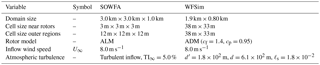
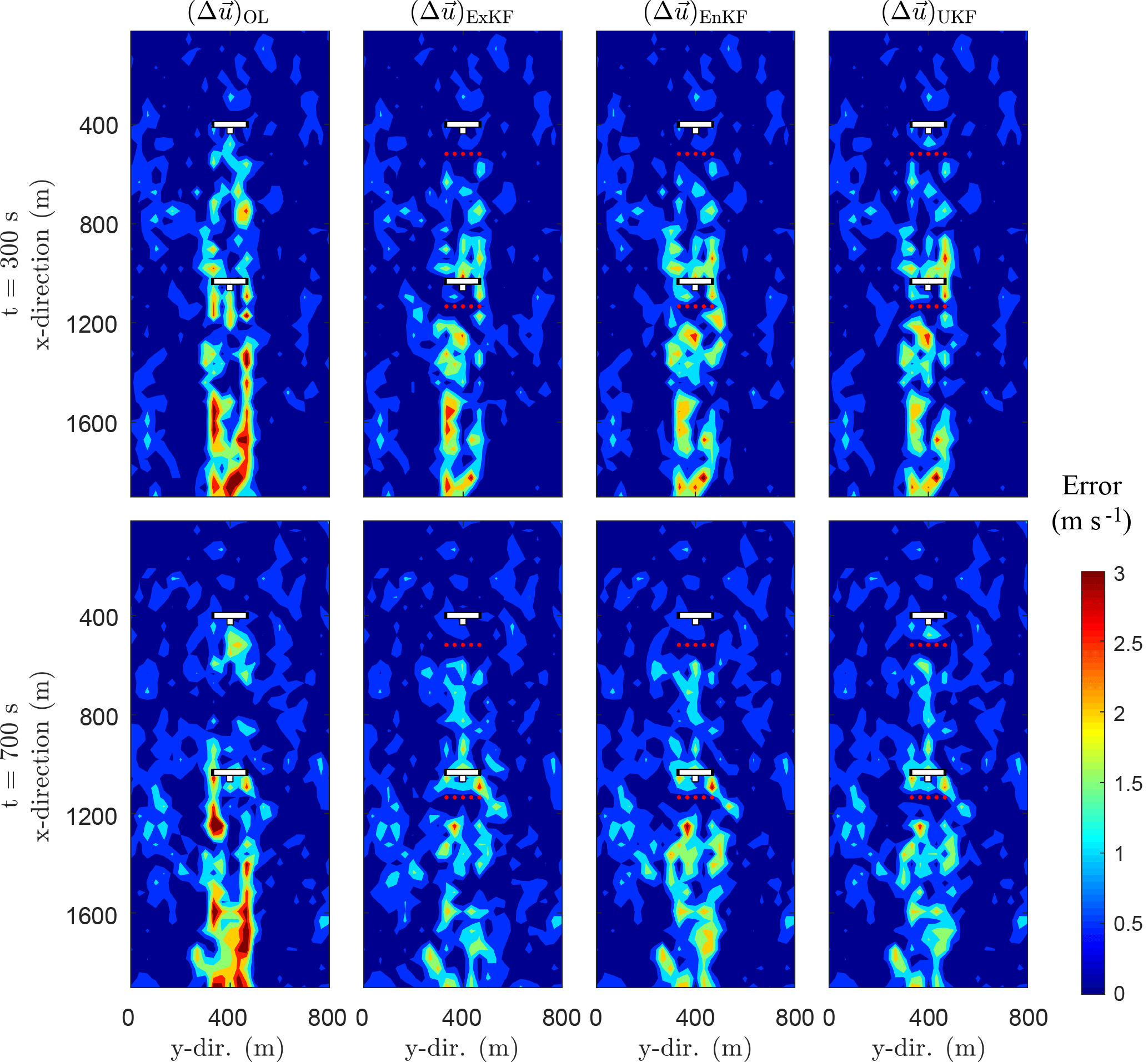
Figure 4Comparison of absolute values of the estimation errors (in long. flow fields) for state-only estimation with the ExKF, EnKF and UKF at t=300 s and t=700 s, with . The model and KF settings are depicted in Tables 1, 2, and 3. Wind is coming in from the top, flowing towards the bottom. The measured states are depicted by red dots in the flow, not to be confused with estimation error. The KFs consistently improve the instantaneous flow field estimations, noticeably nearby the measurements.
4.1 SOWFA
High-fidelity simulation data are generated using the Simulator fOr Wind Farm Applications (SOWFA), developed by the National Renewable Energy Laboratory (NREL). SOWFA provides accurate flow data at a fraction of the cost of field tests. It solves the filtered, three-dimensional, unsteady, incompressible Navier–Stokes equations over a finite temporal and spatial mesh, accounting for the Coriolis and geostrophic forcing terms. SOWFA is a LES solver, meaning that larger-scale dynamics are resolved directly, and turbulent structures smaller than the discretization are approximated using subgrid-scale models to suppress computational cost. (Churchfield et al., 2012). The turbine rotor is modeled using an actuator line representation (ALM) as derived from Sorensen and Shen (2002). SOWFA has previously been used for lower-fidelity model validation, controller testing, and to study the aerodynamics in wind farms (Fleming et al., 2016, 2017a; Gebraad et al., 2017). The interested reader is referred to Churchfield et al. (2012) for a more in-depth description of SOWFA and LES solvers in general.
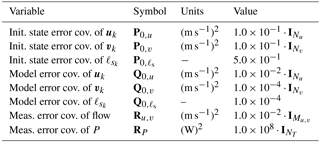
Table 2Covariance settings for the KF variants, with I• the ℝ•×• identity matrix. The full cov. matrices are diagonal concatenations of the entries. For example, P0 is and for state-only and state-parameter estimation, respectively.
4.2 Two-turbine simulation with turbulent inflow
In this section, a two-turbine wind farm is simulated to analyze the effect of different measurement sources, KF algorithms, and the difference between state-only and state-parameter estimation. This simple wind farm contains two NREL 5-MW baseline turbines with D=126.4 m, separated 5D in stream-wise direction. This LES simulation was described in more detail in Annoni et al. (2016). Important simulation properties are listed in Table 1 for SOWFA and WFSim. The effect of the turbulence intensity on the wake dynamics in SOWFA is captured in WFSim through its mixing-length turbulence model. In these simulations, WFSim is purposely initialized with a too low value for ℓs in order to represent the realistic situation of a model mismatch. The remaining tuning parameters in WFSim were chosen such that a weighted-sum cost function of the power and flow errors was minimized.
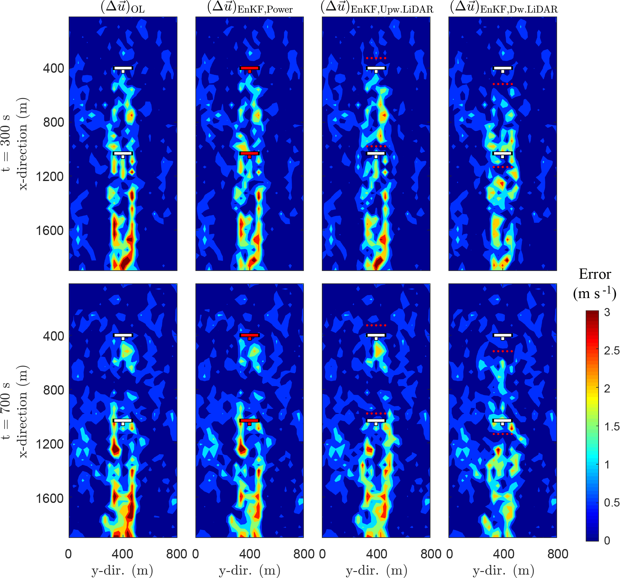
Figure 5Comparison of absolute values of the estimation errors (in long. flow fields) for state-only estimation with the EnKF for various sensor configurations: using turbine power measurements, using flow measurements with a lidar system pointing upstream, and using flow measurements with a lidar system pointing downstream of the rotor. Here, . Here, wind flows from top to bottom. The sensors are depicted by red dots (flow meas.) or red turbines (power meas.), not to be confused with estimation error.
Firstly, the three KF variants will be compared in Sect. 4.2.1. Secondly, in Sect. 4.2.2, estimation using different information sources is compared. Thirdly, the potential of joint state-parameter estimation is displayed in Sect. 4.2.3.
4.2.1 A comparison of the KF variants for state estimation
In this simulation study, four estimation cases are compared: (1) the ExKF, (2) the UKF, (3) the EnKF, and (4) the open-loop (OL) simulation, i.e., without estimation. The focus here is on state-only estimation, thus excluding ℓs. Flow measurements downstream of each turbine are assumed (e.g., using lidar), their locations denoted as red dots in Fig. 4, which is about 2 % of the full to-be-estimated state space. These measurements are artificially disturbed by zero-mean white noise with σ=0.10 m s−1. The KF settings are listed in Tables 2 and 3. The KF covariance matrices were obtained through an iterative tuning process in previous work (Doekemeijer et al., 2017) with minor adjustments to simulate performance for untrained data. Figure 4 shows state (flow field) estimation of the three KF variants for two time instants, t=300 s and t=700 s. In this figure, is defined as the absolute error between the estimated and true longitudinal flow velocities in the field.
Looking at Fig. 4, the OL estimations are accurate for the unwaked and single-waked flow, yet are lacking in the situation of two overlapping wakes, for which the KFs correct. There is no significant difference in accuracy between the different KF variants, yet they differ by 2 orders of magnitude in computational cost (Table 3).
Table 3Choice of tuning parameters for the KF variants, for both the two-turbine and nine-turbine simulation case. Note that the ExKF does not support power measurements nor parameter estimation due to the lack of linearization, and does not have any additional tuning parameters. In terms of computational cost: simulations were run on a single node using 8 cores in parallel.
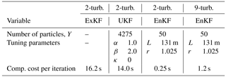
Table 4Overview of several settings for the SOWFA and the WFSim nine-turbine wind farm simulation.
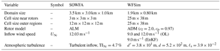

Figure 6Comparison of forecasting performance for state-only and joint state-parameter (ℓs) estimation with the EnKF and UKF, where measurements are available up until the vertical dashed lines, after which the estimation becomes a forecast. Here, the 2-norm of the estimation error is plotted along the y axis, with .
4.2.2 A comparison of sensor configurations
Previous results (Doekemeijer et al., 2016, 2017) have relied on flow measurements for state estimation. However, in existing wind farms, such measurements are typically not available. Rather, readily available SCADA data should be used for the purpose of model calibration. For this reason, state estimation with the EnKF leveraging instantaneous turbine power measurements, using an upstream-pointing lidar, and using a downstream-pointing lidar are compared in Fig. 5. Flow and power measurements are artificially disturbed by zero-mean white Gaussian noise with σ=0.10 m s−1 and σ=104 W, respectively.
The KF settings are displayed in Tables 2 and 3. In Fig. 5 it can be seen that SCADA data allows comparable performance compared to the use of flow measurements, making the proposed closed-loop control solution feasible for implementation in existing wind farms, without the need for additional equipment. Furthermore, this modular framework allows for the use of a combination of lidar systems, measurement towers, and/or SCADA data – whichever is available – for model calibration.
4.2.3 Joint state-parameter estimation
Forecasting, as used in predictive control, benefits from the calibration of model parameters in addition to the states. Joint state-parameter estimation using flow measurements downstream of each turbine (as shown in the rightmost plots in Fig. 5) disturbed by zero-mean white noise with σ=0.10 m s−1 for the EnKF and UKF is displayed in Fig. 6. The KF settings are shown in Tables 2 and 3. At t=0 s, both the OL and the KF simulations start with the same (wrong) value for ℓs. Then, every second, (noisy) measurements are fed into the KFs, and the state vector as well as the model parameter ℓs is estimated. However, for the OL simulation, no measurements are fed in: the state vector is simply updated with the nominal model, and the value for ℓs remains the same throughout the simulation. Now, after 600 s (left plot in Fig. 6) and 900 s (right plot in Fig. 6), a forecast is started, meaning no measurements are available after that time. At that moment, the OL model still has the same (poor) value for ℓs as at t=0 s, while the value for ℓs in the KFs has improved. From Fig. 6, it becomes clear that the estimates are not only improved for the 3 min forecast, but are also consistently better than the non-calibrated (open-loop) model's 10 min forecast due to the estimation of ℓs3. Furthermore, the EnKF performs comparably to the UKF at a lower computational cost. Note that the EnKF even outperforms the UKF in this simulation, expected to be due to randomness in the EnKF.
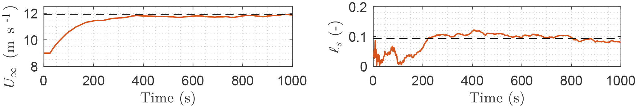
Figure 7Convergence of ℓs and U∞ using the EnKF. Dashed lines are the grid-searched optimal constant values for the open-loop simulation. With power measurements only, the EnKF is able to estimate these parameters successfully in addition to the model states.
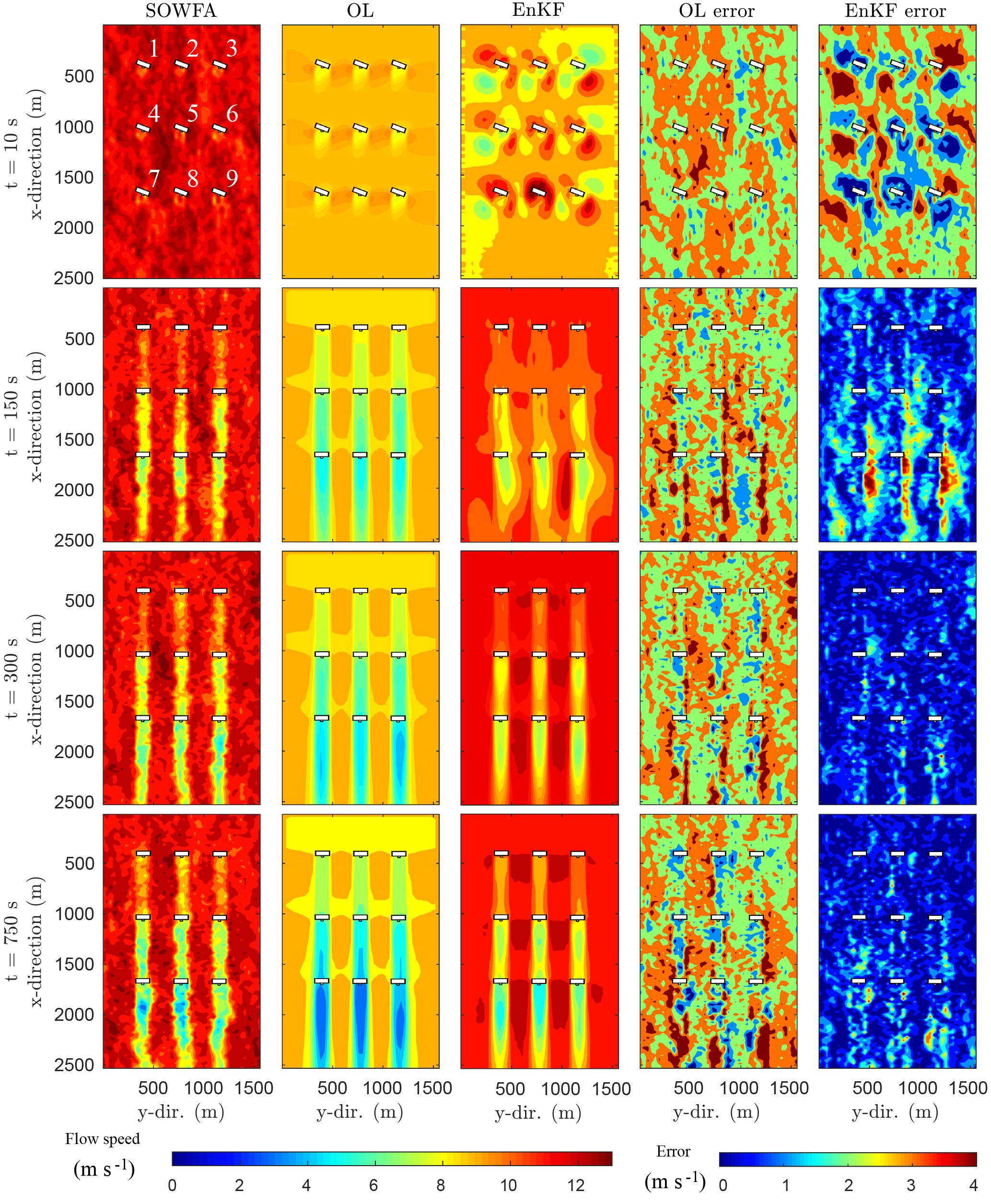
Figure 8Comparison of absolute values of the estimation errors (in long. flow fields) for state-parameter estimation with the EnKF. Wind is coming in from the top and flows downwards. The variables U∞ and ℓs are incorrectly initialized in both the OL and the EnKF. In the EnKF, U∞ and ℓs are estimated in addition to the states, using only turbine power measurements. The EnKF quickly converges for the states, and more slowly for ℓs and U∞. After 300 s, the EnKF has converged to a negligible estimation error.
4.3 Nine-turbine simulation with turbulent inflow
In this section, we investigate the performance of the EnKF-based model calibration solution under a more realistic nine-turbine wind farm scenario. The purpose of this case study is to highlight the need for state-parameter estimation for accurate wind farm modeling. The wind farm contains nine NREL 5-MW baseline turbines, oriented in a three by three layout, separated 5D and 3D in stream- and crosswise directions, respectively. The turbines start with a 30∘ yaw misalignment, but are then aligned with the mean wind direction within the first 30 s of simulation. The turbine layout and numbering is shown in the top-left panel of Fig. 8. This LES simulation has been used before in the literature, and is described in more detail in Boersma et al. (2018). A number of important simulation properties are listed in Table 4 for SOWFA and WFSim, respectively.

Figure 9Comparison of power forecasting using the EnKF with measurements available up until time t=600 s. After convergence U∞ (as seen as a positive power slope for the first row of turbines), ℓs is also calibrated. After convergence, forecasting is better than in open-loop. Oscillatory behavior is still present due to an oscillatory input signal (), turbulent flow field, and the absence of inertia in the rotor model.
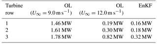
Table 5Turbine-averaged RMSE in power time series of Fig. 9 (compared to SOWFA). The lower the RMSE, the better the forecast.
Compared to the two-turbine case, N has increased by a factor of 4. In the UKF, this would result in the same factor of additional particles. Thus, not only is each particle more expensive to calculate but there are also more particles. Rather, in the EnKF, the approach is heuristic. None of the EnKF settings needed to be changed for good performance compared to Sect. 4.2, as displayed in Tables 2 and 3.
As shown in Table 3, the EnKF has a low computational cost of 1.2 s per iteration (8 cores, parallel). In this case study, both the complete model state (flow field), the turbulence model parameter ℓs, and the free-stream flow speed U∞ are estimated in real-time using exclusively (readily available) power measurements from the turbines. The EnKF and one of the open-loop simulations (OL) will deliberately be initialized with poor values for ℓs and U∞ to investigate convergence. The other OL simulation will be initialized with a poor value for ℓs but a correct value for U∞ for comparison.
In Fig. 7, it can be seen that the EnKF is successful in estimating U∞ and ℓs after 300 s using only wind turbine power measurements. Furthermore, the flow fields of SOWFA, of the OL simulation with U∞=9.0 m s−1, and of the EnKF at various time instants are displayed in Fig. 8. From this figure, it can be seen that the EnKF has large errors at the start of the simulation. However, after 10 s, the error in flow states surrounding each turbine significantly decreases through the use of turbine power measurements. This estimated flow then propagates downstream, “clearing up” the errors in the vicinity of the wind turbines. As time further propagates, the free-stream estimation improves, and finally the estimation error converges.
The power forecasting performance is shown in Fig. 9 and Table 5. As also seen in Fig. 7, the EnKF converges after 300 s, and indeed the power forecasts outperform those of the OL simulation at t=300 s. Furthermore, it is interesting to see that the filtered power estimates of the first row of turbines (i=1, 2, 3) starts low at t=1 s, but converges to the true power at t≈200 s. This can be related to the mismatch in U∞, which takes approximately 300 s to converge to the true value of 12 m s−1, as seen in Fig. 7. The oscillatory behavior in both the OL and EnKF power predictions is due to the absence of rotor inertia in the rotor model, turbulent structures in the flow, and large fluctuations on the excitation signal .
Finally, the forecasts for flow at times t=300 s and t=600 s are examined in Fig. 10. The large flow estimation mismatch in the EnKF at t<250 s quickly reduces and for t≥250 s the EnKF estimation is consistently better than both the OL cases. This has to do with the convergence of the model parameters ℓs and U∞, and the estimation of the states surrounding the turbines using the power measurements.
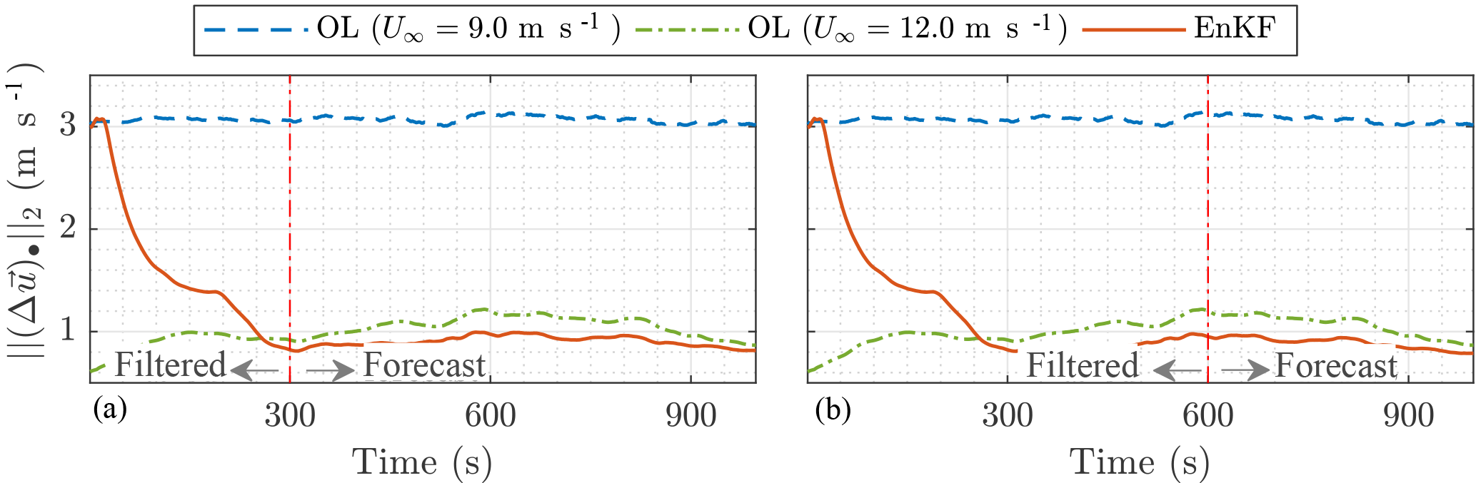
Figure 10Comparison of flow field estimation for the nine-turbine case. Measurements are available until t=300 s (a) and t=600 s (b), respectively. The EnKF converges to the true U∞ after 300 s. After convergence, the forecasts are significantly better than in open-loop simulations.
A crucial remark with the simulations presented here is that low-frequency changes in the atmosphere are neglected. In a real wind farm, atmospheric properties such as the mean wind direction and turbulence intensity change continuously, and this will impact the estimation and forecasting performance. The EnKF uses an assumption of persistence for the atmospheric properties at the time of forecasting, and thus a change in mean wind direction may invalidate the model forecast. In future work, the algorithm presented here should be tested under high-fidelity simulations with such realistic low-frequency changes. This would provide insight into the potential of the work at hand, and advance towards a practical wind farm implementation.
This paper presented a real-time model calibration algorithm for the dynamic wind farm model “WFSim”, relying on an ensemble Kalman filter (EnKF) at its core. The joint state-parameter calibration solution was tested in two high-fidelity simulation case studies. Exclusively using SCADA measurements, which are readily available in current wind farms, the adaptability to model discrepancies in a nine-turbine wind farm simulation was shown, at a low computational cost of 1.2 s per time step on an eight-core CPU. Specifically, the free-stream wind speed and turbulence intensity were shown to converge to their optimal values within 300 s. Furthermore, the EnKF was shown to perform comparably in terms of accuracy to the state-of-the-art algorithms in the literature, at a computational cost of multiple orders of magnitude lower. Additionally, estimation using flow measurements from lidar was compared to estimation using SCADA data, and it was shown that SCADA data can effectively be used for real-time model calibration. In future work, the algorithm presented here should be tested under high-fidelity simulations with realistic low-frequency changes. This would provide insight into the potential of the work at hand, and advance towards a practical wind farm implementation. This work presented an essential building block for real-time closed-loop wind farm control using surrogate dynamic wind farm models.
The surrogate model and estimation solutions presented in this article are open-source software, available at https://github.com/tudelft-datadrivencontrol (last access: 7 September 2018). SOWFA is available at https://github.com/NREL/SOWFA (last access: 5 July 2018). All rights for SOWFA and the simulation data presented in this work belong to the National Renewable Energy Laboratory.
The authors declare that they have no conflict of interest.
The authors thank Matti Morzfeld for the insightful discussions concerning
the ensemble Kalman filter. However, any mistakes in this work remain the
authors' own. This project has received funding from the European Union's
Horizon 2020 research and innovation program under grant agreement no. 727477.
Edited by: Carlo L. Bottasso
Reviewed by: two anonymous referees
Aho, J., Buckspan, A., Laks, J., Fleming, P. A., Jeong, Y., Dunne, F., Churchfield, M., Pao, L. Y., and Johnson, K.: A tutorial of wind turbine control for supporting grid frequency through active power control, American Control Conference (ACC), 3120–3131, Piscataway, New Jersey, USA, 2012. a
Annoni, J., Gebraad, P. M. O., and Seiler, P.: Wind farm flow modeling using an input-output reduced-order model, American Control Conference (ACC), 506–512, Piscataway, New Jersey, USA, 2016. a
Boersma, S., Doekemeijer, B. M., Gebraad, P. M. O., Fleming, P. A., Annoni, J., Scholbrock, A. K., Frederik, J. A., and van Wingerden, J. W.: A tutorial on control-oriented modeling and control of wind farms, American Control Conference (ACC), 1–18, Piscataway, New Jersey, USA, 2017. a, b, c
Boersma, S., Doekemeijer, B., Vali, M., Meyers, J., and van Wingerden, J.-W.: A control-oriented dynamic wind farm model: WFSim, Wind Energ. Sci., 3, 75–95, https://doi.org/10.5194/wes-3-75-2018, 2018. a, b, c, d, e, f, g, h, i, j
Churchfield, M. J., Lee, S., Michalakes, J., and Moriarty, P. J.: A numerical study of the effects of atmospheric and wake turbulence on wind turbine dynamics, J. Turbul., 13, 1–32, 2012. a, b
Doekemeijer, B. M., van Wingerden, J. W., Boersma, S., and Pao, L. Y.: Enhanced Kalman filtering for a 2D CFD NS wind farm flow model, J. Phys. Conf. Ser., 753, https://doi.org/10.1088/1742-6596/753/5/052015, 2016. a, b, c, d
Doekemeijer, B. M., Boersma, S., Pao, L. Y., and van Wingerden, J. W.: Ensemble Kalman filtering for wind field estimation in wind farms, American Control Conference (ACC), 19–24, Piscataway, New Jersey, USA, 2017. a, b, c, d, e, f, g
Ela, E., Gevorgian, V., Fleming, P. A., Zhang, Y. C., Singh, M., Muljadi, E., Scholbrock, A. K., Aho, J., Buckspan, A., Pao, L. Y., Singhvi, V., Tuohy, A., Pourbeik, P., Brooks, D., and Bhatt, N.: Active power controls from wind power: bridging the gaps, Tech. Rep. NREL/TP-5D00-60574, National Renewable Energy Laboratory, 2014. a
Evensen, G.: The Ensemble Kalman Filter: theoretical formulation and practical implementation, Ocean Dynam., 53, 343–367, 2003. a
Fleming, P. A., Aho, J., Gebraad, P. M. O., Pao, L. Y., and Zhang, Y.: Computational fluid dynamics simulation study of active power control in wind plants, American Control Conference (ACC), 1413–1420, Piscataway, New Jersey, USA, 2016. a, b
Fleming, P. A., Annoni, J., Scholbrock, A. K., Quon, E., Dana, S., Schreck, S., Raach, S., Haizmann, F., and Schlipf, D.: Full-scale field test of wake steering, J. Phys. Conf. Ser., 854, 012013, https://doi.org/10.1088/1742-6596/854/1/012013, 2017a. a, b
Fleming, P., Annoni, J., Shah, J. J., Wang, L., Ananthan, S., Zhang, Z., Hutchings, K., Wang, P., Chen, W., and Chen, L.: Field test of wake steering at an offshore wind farm, Wind Energ. Sci., 2, 229–239, https://doi.org/10.5194/wes-2-229-2017, 2017b. a
Gaspari, G. and Cohn, S. E.: Construction of correlation functions in two and three dimensions, Q. J. Roy. Meteor. Soc., 125, 723–757, 1999. a
Gebraad, P., Thomas, J. J., Ning, A., Fleming, P. A., and Dykes, K.: Maximization of the annual energy production of wind power plants by optimization of layout and yaw-based wake control, Wind Energy, 20, 97–107, 2017. a
Gebraad, P. M. O. and van Wingerden, J. W.: Maximum power-point tracking control for wind farms, Wind Energy, 18, 429–447, 2015. a
Gebraad, P. M. O., Fleming, P. A., and van Wingerden, J. W.: Wind turbine wake estimation and control using FLORIDyn, a control-oriented dynamic wind plant model, American Control Conference (ACC), 1702–1708, Piscataway, New Jersey, USA, 2015. a
Gebraad, P. M. O., Teeuwisse, F. W., van Wingerden, J. W., Fleming, P. A., Ruben, S. D., Marden, J. R., and Pao, L. Y.: Wind plant power optimization through yaw control using a parametric model for wake effects – a CFD simulation study, Wind Energy, 19, 95–114, 2016. a, b, c
Gillijns, S., Mendoza, O. B., Chandrasekar, J., De Moor, B. L. R., Bernstein, D. S., and Ridley, A.: What is the ensemble Kalman filter and how well does it work?, American Control Conference (ACC), 4448–4453, Piscataway, New Jersey, USA, 2006. a
Goit, J. P. and Meyers, J.: Optimal control of energy extraction in wind-farm boundary layers, J. Fluid Mech., 768, 5–50, 2015. a
Houtekamer, P. L. and Mitchell, H. L.: Ensemble Kalman filtering, Q. J. Roy. Meteor. Soc., 131, 3269–3289, 2005. a
International Energy Agency: World Energy Outlook 2017, Tech. rep., International Energy Agency, London, England, UK, 2017. a
Iungo, G. V., Santoni-Ortiz, C., Abkar, M., Porté-Agel, F., Rotea, M. A., and Leonardi, S.: Data-driven reduced order model for prediction of wind turbine wakes, J. Phys. Conf. Ser., 625, https://doi.org/10.1088/1742-6596/625/1/012009, 2015. a
Kalman, R. E.: A new approach to linear filtering and prediction problems, J. Basic Eng.-T. ASME, 82, 35–45, 1960. a
Knudsen, T., Bak, T., and Svenstrup, M.: Survey of wind farm control – power and fatigue optimization, Wind Energy, 18, 1333–1351, 2015. a
Mittelmeier, N., Blodau, T., and Kühn, M.: Monitoring offshore wind farm power performance with SCADA data and an advanced wake model, Wind Energ. Sci., 2, 175–187, https://doi.org/10.5194/wes-2-175-2017, 2017. a
Munters, W. and Meyers, J.: An optimal control framework for dynamic induction control of wind farms and their interaction with the atmospheric boundary layer, Philos. T. Roy. Soc. A, 375, https://doi.org/10.1098/rsta.2016.0100, 2017. a, b, c, d
Petrie, R. E.: Localization in the Ensemble Kalman filter, Master's dissertation, University of Reading, 2008. a, b
Rotea, M. A.: Dynamic programming framework for wind power maximization, IFAC Proceedings Volumes, 47, 3639–3644, 19th IFAC World Congress, Elsevier, Amsterdam, the Netherlands, 2014. a, b
Schreiber, J., Nanos, E. M., Campagnolo, F., and Bottasso, C. L.: Verification and calibration of a reduced order wind farm model by wind tunnel experiments, J. Phys. Conf. Ser., 854, https://doi.org/10.1088/1742-6596/854/1/012041, 2017. a
Shapiro, C. R., Bauweraerts, P., Meyers, J., Meneveau, C., and Gayme, D. F.: Model-based receding horizon control of wind farms for secondary frequency regulation, Wind Energy, 20, 1261–1275, Piscataway, New Jersey, USA, 2017a. a, b, c
Shapiro, C. R., Meyers, J., Meneveau, C., and Gayme, D. F.: Dynamic wake modeling and state estimation for improved model-based receding horizon control of wind farms, American Control Conference (ACC), 709–716, Piscataway, New Jersey, USA, 2017b. a
Simley, E. and Pao, L. Y.: Evaluation of a wind speed estimator for effective hub-height and shear components, Wind Energy, 19, 167–184, 2016. a
Siniscalchi-Minna, S., Bianchi, F. D., and Ocampo-Martinez, C.: Predictive control of wind farms based on lexicographic minimizers for power reserve maximization, American Control Conference (ACC), Piscataway, New Jersey, USA, 2018. a
Sorensen, J. N. and Shen, W. Z.: Numerical modeling of wind turbine wakes, J. Fluid Mech., 124, 393–399, 2002. a
Vali, M., Petrović, V., Boersma, S., Van Wingerden, J. W., and Kühn, M.: Adjoint-based model predictive control of wind farms: Beyond the quasi steady-state power maximization, IFAC World Congress, 50, 4510–4515, 2017. a, b, c, d
Van Wingerden, J. W., Pao, L. Y., Aho, J., and Fleming, P. A.: Active power control of waked wind farms, IFAC World Congress, 4570–4577, https://doi.org/10.1016/j.ifacol.2017.08.378, 2017. a
Wan, E. A. and Van Der Merwe, R.: The unscented Kalman filter for nonlinear estimation, Proceedings of the IEEE Adaptive Systems for Signal Processing, Communications, and Control Symposium, 153–158, Piscataway, New Jersey, USA, 2000. a, b, c, d, e
Note that it is still uncertain what accuracy is necessary and what computational cost can be permitted for real-time closed-loop wind farm control.
Note that this method for the estimation of U∞ relies solely on power measurements, and therefore only works for below-rated conditions. For estimation of U∞ in above-rated conditions, one may require the implementation of a wind speed estimator on each turbine (e.g., Simley and Pao, 2016).
Note that this is highly dependent on the frequency at which the free-stream conditions change in the atmosphere.