2.1 Wake model

We used the FLORIS wake model to predict the wind speeds throughout the wind farms in our study (Gebraad et al., 2016). The FLORIS model had some discontinuities in the original formulation, so in this study we used a version that has been modified to be smooth and continuously differentiable, enabling gradient-based optimization (Thomas et al., 2017). Additionally, we use a version of the FLORIS wake model that has been modified to consider the 3-D flow field in the wind farm instead of a simpler 2-D flow field (Stanley et al., 2019).

The total velocity deficit, L, at any given point was defined as the square root of the sum of the squares of the loss contribution from each turbine wake, l_i:

Variations in the free-stream wind speed with height were calculated with the wind profile power law:

where V is the wind speed at height z; V_ref is the reference wind speed given by the wind data; z_ref is height at which the reference wind speed was measured, which we assumed to be 50 m; and α is the wind shear exponent, which defines how the wind speed varies with height.

2.2 Annual energy production calculation

2.2.2 Wind speed distributions

We represented the speeds at any wind direction as a Weibull distribution, which is commonly used to represent wind speed distributions (Justus et al., 1978; Rehman et al., 1994; Dorvlo, 2002):

$$\begin{array}{}\text{(5)}& W\left(V\right)=\left({\displaystyle \frac{k}{V_{\mathrm{mean}}}}\right)\left({\displaystyle \frac{V}{V_{\mathrm{mean}}}}{)}^{k-\mathrm{1}}\exp \right[(-{\displaystyle \frac{V}{V_{\mathrm{mean}}}}{)}^k].\end{array}$$

This equation defines the frequency (W) of a certain wind speed (V). The shape factor, k, was set to 1.76, which is in the range of realistic shape factors fit to real wind data from various sites around the world (Garcia et al., 1998; Lun and Lam, 2000). The mean speed for a given distribution, V_mean, could be different depending on the wind direction, meaning that each wind direction had an associated Weibull curve defining the wind speed distribution from that direction. Figure 1 shows the wind speed Weibull distributions for two different V_mean values.

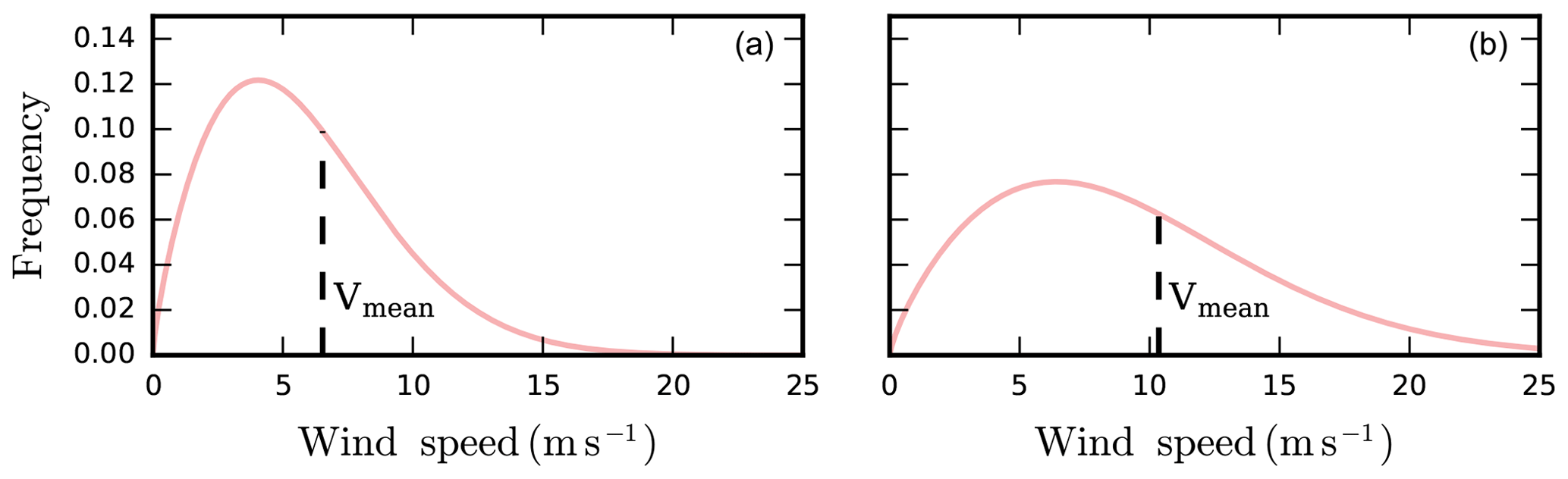
Figure 1The Weibull wind speed distributions for two different average wind speeds. In (a) there is an average wind speed of 6.53 m s⁻¹, and (b) shows an average wind speed of 10.35 m s⁻¹. The shape factor k in each Weibull distribution was chosen as 1.76.

Download

2.3 Tower model

Because the tower height varied in this study, it was necessary to calculate the tower mass and perform structural analyses. In the structural analysis, we calculated stress and buckling in the tower and constrained these values during the optimization. It was necessary to provide a model with gradients for all of our constraints, which included the von Mises stress, shell buckling, and global buckling at any point along the tower; the tower taper ratio; and the first natural frequency of the structure. The method by which these calculations were made is discussed in more detail in our previous study (Stanley et al., 2019).

2.4 Rotor/nacelle models

The variable rotor diameter, turbine power rating, and blade and chord distributions in this study also needed be accounted for in structural analysis. To do so, we used a model developed at the National Renewable Energy Laboratory (NREL) called RotorSE to calculate the rotor mass, rated and extreme thrust, rated torque, rated wind speed, and moments of inertia (Ning, 2013). The complex nature of RotorSE allows the user to fully define a rotor and perform analysis; however, this comes at a cost in computation time. Because we coupled turbine design and turbine layout optimization, the rotor analysis needed to be called many more times than in an isolated turbine design optimization. Thus, to speed up the rotor calculations in our optimization, we created a surrogate model on the results provided by RotorSE. We sampled rotor diameters evenly spaced from 46 to 160 m, every 6 m, and rated powers from 0.5 to 10 MW, every 0.5 MW. The lower limits – 46 m rotor diameter and 500 kW rated power – are both lower than we expected any of the optimal values to be. The upper limits – 160 m rotor diameter and 10 MW rated power – are both near the upper limit of current wind turbine technology. For each combination of rotor diameter and rated power, we used RotorSE to minimize the blade mass using the blade chord-and-twist distributions as design variables. The optimization was constrained such that the turbine blades would not fail from stress or buckling and the power coefficient was greater than 0.42. Note that we did not vary the airfoils in the optimizations but used those defined by the NREL 5 MW reference turbine (Jonkman et al., 2009). We then used the converged optimizations, and used k-fold cross validation with 10 groups to choose a fifth-order bivariate spline, which was then applied to each of the outputs of interest. This spline function was then used in place of RotorSE in our wind farm optimizations. By creating the surrogate, we achieved the accuracy of RotorSE without the large associated time requirement, as well as fast and simple analytic gradients. The k-fold cross validation with 10 groups showed that the mean error is below 4 % for the moments of inertia, approximately 4.5 % for the extreme thrust, and below 3 % for the rest of the fits. Figure 2 shows the normalized surface fits for each of the variables of interest.

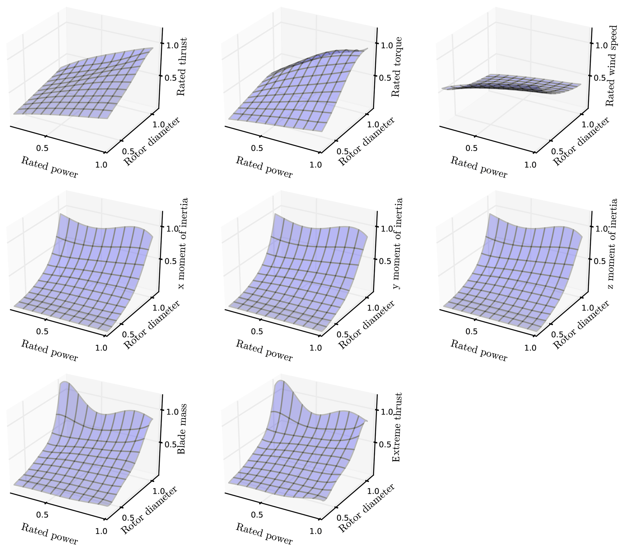
Figure 2The spline fits to optimized RotorSE data. These fits were used to obtain the desired outputs of rotor mass, rated and extreme thrust, rated torque, rated wind speed, and moments of inertia as functions of the rotor diameter and rated power.

Download

2.5 Cost model

AEP is a standard objective in wind farm optimization problems because it is easy to calculate and is a valid measure when only power production is affected by the optimization. When aspects of turbine design are included as design variables, this measure is no longer appropriate because costs of the wind farm are affected as well. To accurately represent the trade-offs between power production and cost, we evaluated our wind farm by its COE as was done in our previous paper on wind farms with different turbine heights (Stanley et al., 2019).

2.6 Optimization

We set up our optimization with two different turbine groups. We assigned each turbine to one of two groups, where all turbines in a group had the same tower hub height, rotor diameter, turbine rating, tower diameter, tower shell thickness, and blade chord-and-twist distributions. Rather than optimize each turbine, we chose two groups because our previous study in which we optimized wind farms with different turbine heights indicated that the most benefit comes from increasing from one height group to two. Any benefit from introducing more groups was insignificant (Stanley et al., 2019). We parameterized the tower by specifying the diameter and shell thickness at the bottom, midpoint, and top of the tower and then linearly interpolating diameter and shell thickness at points in between, as shown in Fig. 3.

It may be beneficial to do a binary optimization in which each turbine can change the turbine group to which it belongs, but this greatly increases the complexity of the optimization and makes it gradient-free. Gradient-free optimization is more computationally expensive, which severely limits the number of design variables we can include in the problem. To maintain the gradient-based optimization, we assigned each turbine to one of the groups before starting the optimization. Although the turbines could move throughout the wind farm, once assigned a turbine could not switch to the other group. In this study, we only examined an equal weighting of turbines in each group, but additional benefit may come from optimally choosing the number of turbines in each group.

We ran several cases in which different design variables were included in the problem to allow comparison of their effects on COE. In all, the design variables we included were the position of each turbine (x_i, y_i), the tower height of each group (H₁, H₂), the rotor diameter of each group (D₁, D₂), the rated power of each group (R₁,R₂), the tower diameter of each group (d_1,j, d_2,j), and the tower shell thickness of each group (t_1,j, t_2,j). Index j refers location on the tower (j=1 is at the bottom, j=2 at the midpoint, j=3 at the top), meaning there are six total variables to define diameter (three for each height group) and six to define the tower shell thickness. The blade chord-and-twist distributions also varied during the optimization; however, because these were optimized separately to minimize mass when creating our rotor surrogate model, they were not explicitly changed in this part of the optimization, making them implicit design variables.

The turbine layout and structural constraints were previously formulated in our multiple-hub-height study (Stanley et al., 2019). Because rotor diameter was a design variable, the turbine spacing constraint was slightly reformulated such that the distance between any two turbines in the wind farm was greater than the sum of the two rotor diameters. Shell buckling refers to the buckling of the cylindrical turbine tower, or hollow “shell”. The margins are unit-less and can be expressed as

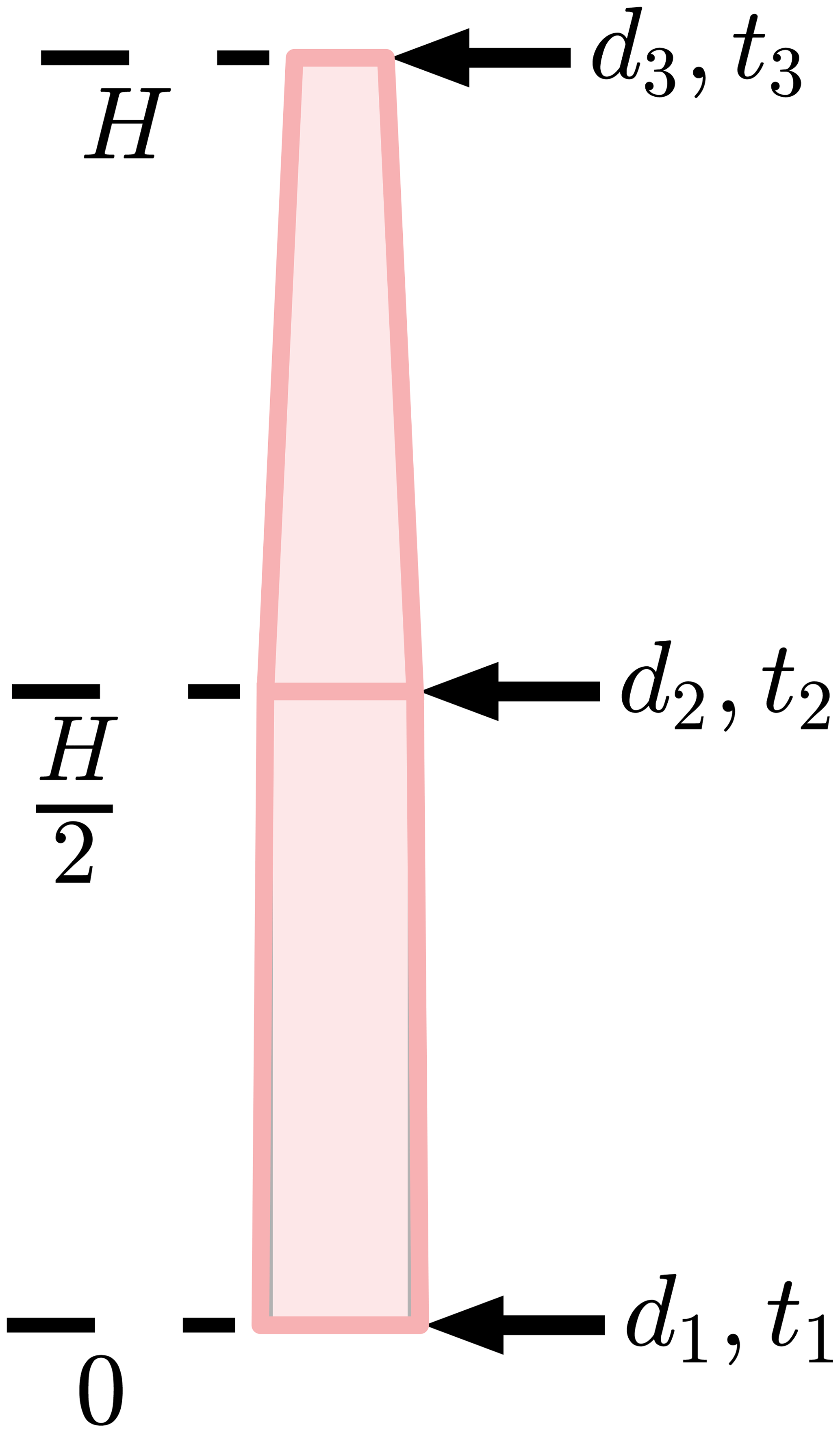
Figure 3The parameterized turbine tower definition. The tower diameter and shell thickness are defined at the bottom, midpoint, and top of the tower, with the values linearly interpolated in between.

Download

The rotor diameter and the turbine rating were constrained by the lowest and highest values that were included in the RotorSE optimization, as discussed in Sect. 2.4. The lower limits were never active in these optimizations; however, some of the upper limits were active, as will be seen in the “Results” section. The optimization can be expressed as follows:

Note that i is the index defining the wind turbine and j is the index describing the location on the tower.

The gradients for this optimization were all analytic. We calculated the partial derivatives of each small section of the model and included each part in a framework called OpenMDAO, which calculated the gradients of the entire system (Gray et al., 2010). The analytic gradients were significant because they were more accurate, converged to better solutions, and converged on the solution much faster than finite difference gradients. More importantly, they allowed us to solve much larger optimization problems than would have been possible without.

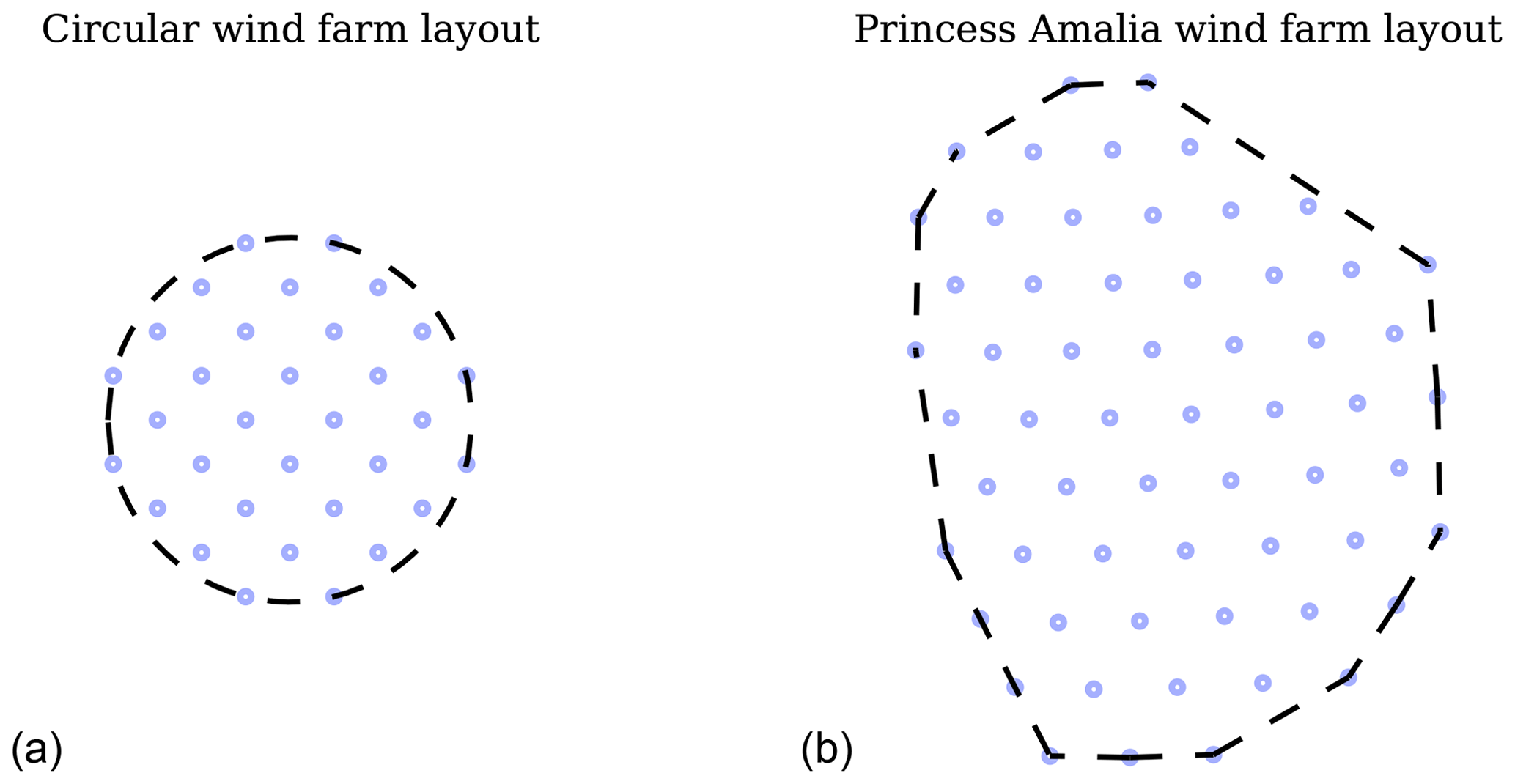
Figure 4The two different wind farm designs that were optimized: (a) is a contrived circular wind farm design with 32 turbines; (b) is the Princess Amalia wind farm, an offset grid design with 60 wind turbines. The circles representing the turbine locations have a diameter of 80 m in this figure, equal to the baseline rotor diameter.

Download

We optimized two different wind farms, each with several different wind shear exponents and turbine spacing multipliers as will be explained later in this section. The first wind farm was an imagined 32-turbine wind farm with a circular boundary, shown in Fig. 4. This wind farm was optimized with wind data from the city of Alturas, California, gathered by Iowa State University, shown in Fig. 5 (https://mesonet.agron.iastate.edu/sites/windrose.phtml?station=AAT&network=CA_ASOS, last access: 25 January 2019). For this wind rose, the average wind speed, V_mean, from each direction of this wind rose was assumed to be 8 m s⁻¹, shown in Fig. 6. The second wind farm was based on the Princess Amalia wind farm, a real farm off the coast of the Netherlands which has 60 wind turbines, and is shown in Fig. 4. This wind farm was optimized with the wind direction and average directional speed data from the NoordzeeWind meteorological mast located in the North Sea, shown in Figs. 5 and 6 (Brand et al., 2012). The farm boundary for the Princess Amalia wind farm was the convex hull of the original Princess Amalia layout. The turbines in the Princess Amalia wind farm are Vestas 2 MW wind turbines, which have a rotor diameter of 80 m. Therefore, for both wind farms we used a baseline rotor diameter of 80 m and a baseline power rating of 2 MW. The baseline hub height used in this study was 100 m.

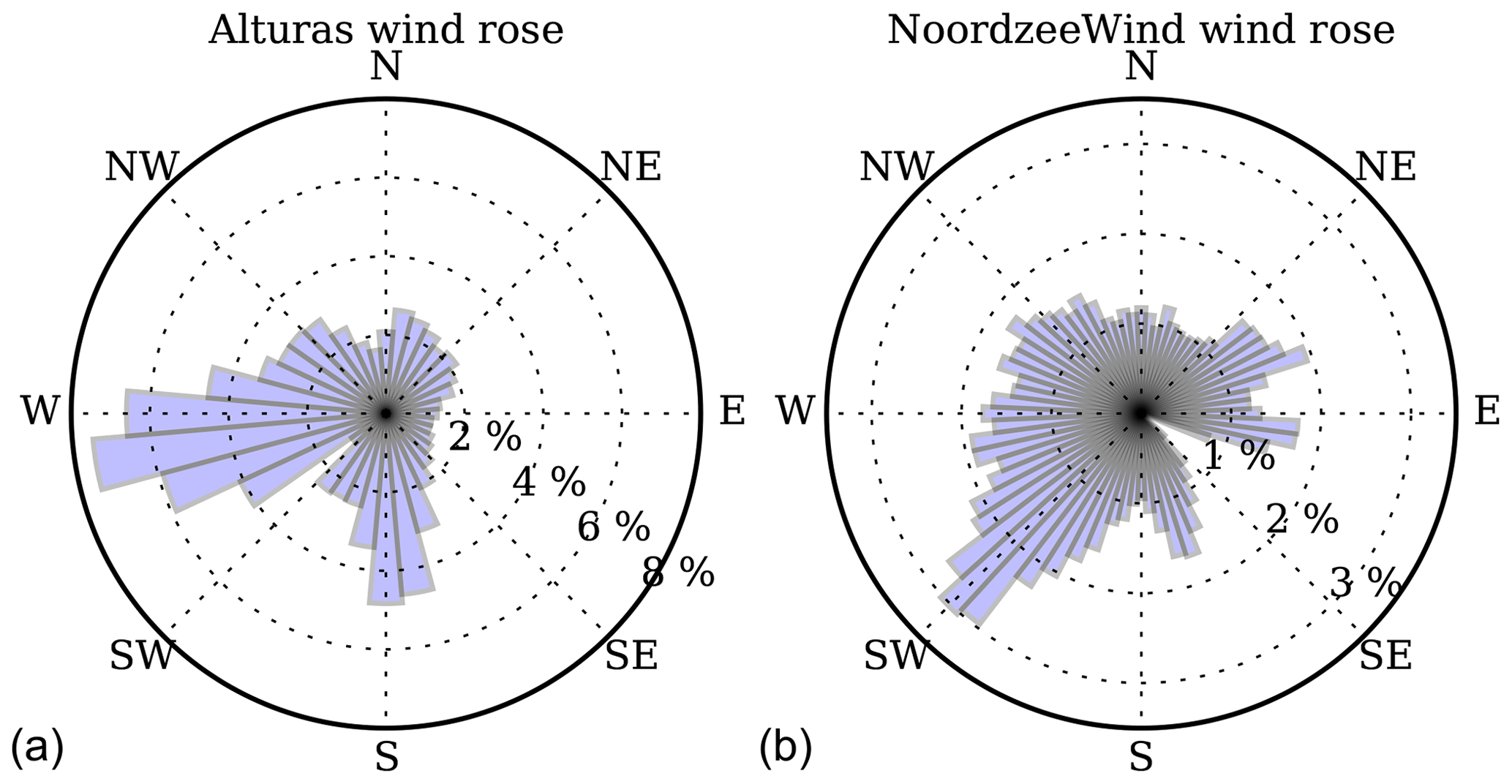
Figure 5Panel (a): the wind direction distribution in Alturas, California, separated into 36 bins, every 10^∘. Panel (b): the wind direction distribution of the NoordzeeWind meteorological mast, separated into 72 bins, every 5^∘.

Download

Figure 6Panel (a): the assumed directionally averaged wind speeds for Alturas, California, separated into 36 bins, every 10^∘. Each direction is assumed to have an average wind speed of 8 m s⁻¹. Panel (b): the directionally averaged wind speeds of the NoordzeeWind meteorological mast, separated into 72 bins, every 5^∘.

Download

We optimized both of the wind farms shown in Fig. 4 with three different wind shear exponents (0.075, 0.175, 0.275) and three different spacing multipliers (0.5, 1.0, 1.5). The wind shear exponent defines how fast the wind speed changes with height, as seen in Eq. (2). Low shear exponents are typical over open water or flat plains, while higher shear exponents exist in areas with obstructions, such as large trees or buildings. Figure 7 shows the wind speed profiles of the three shear exponents we used. For a shear exponent of 0.075, there is only an 8.6 % increase in the wind speed from the reference height of 50 to 150 m. For a shear exponent of 0.175 there is a wind speed increase of 21.2 % for the same height difference, and for a shear exponent of 0.275 the wind speed increase is 35.3 % from 50 to 150 m.

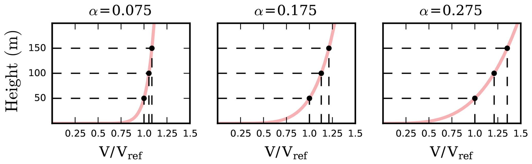
Figure 7The wind speed profiles for various wind shear exponents. With lower shear exponents the wind speed does not vary dramatically with height. For higher wind shear, there is a significant wind speed increase with height.

Download

We also optimized each wind farm for different turbine spacings by adjusting the wind farm size by a spacing multiplier, β. The baseline turbine locations were adjusted to scale with the varied wind farm sizes. The boundary radius of the circular wind farm was multiplied by the spacing multiplier, and the convex hull of the Princess Amalia farm was applied to the baseline turbine locations that had been multiplied by the spacing multiplier. Figure 8 shows both of the wind farms adjusted by the spacing multipliers, as well as the turbine spacing in baseline rotor diameters. The circles represent the turbine locations in this figure, with the circle diameter equal to the baseline rotor diameter, 80 m. As the turbine designs were optimized, the spacings indicated in this figure (in rotor diameters) increased or decreased according to the new rotor diameters. Note that in the circular wind farm, the turbine distances are presented in the rows closely inline with the dominant wind direction (10^∘ south of west; see Fig. 5). The closest neighboring turbines are actually $\sqrt{\mathrm{2}}/\mathrm{2}$ multiplied by this value.

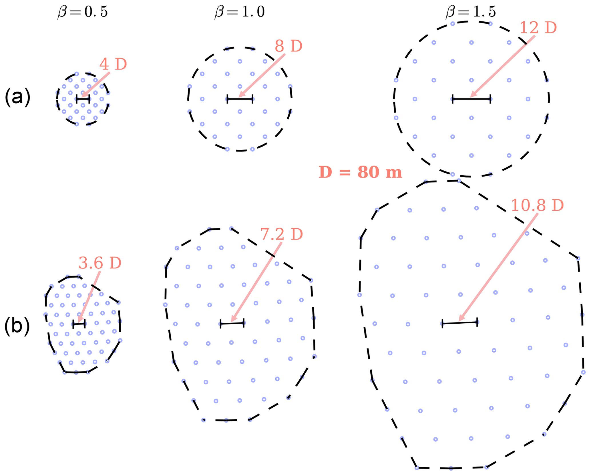
Figure 8The six wind farm boundaries and associated baseline layouts optimized in this study. The same two layouts were multiplied by a spacing multiplier, β=0.5, 1.0, and 1.5, which changed the wind farm size and the average spacing between wind turbines. Panel (a) is the 32-turbine, circular wind farm, and panel (b) is the 60-turbine, Princess Amalia wind farm. The turbine spacings, in baseline rotor diameters, are also displayed for each spacing multiplier in this figure. The circles representing the turbine locations have a diameter of 80 m in this figure, equal to the baseline rotor diameter.

Download

The results of gradient-based optimization, especially for problems with many local minima, are sensitive to the starting location. As in most optimization problems, there is no guarantee that the solution is the global solution. Good results can be achieved with a multiple-start approach, where several different starting points are used for each condition, and the best solution is used. In our study, we ran fifty to hundreds of starting locations for each optimization case. For every optimization, we started each turbine location from the Princess Amalia or circular wind farm baseline locations in Fig. 8, each perturbed randomly up to two baseline rotor diameters in the x and y coordinates. All of the other design variables were initialized randomly for each optimization.

3.1 Circular wind farm

Figure 9 shows the optimal COE results for the circular wind farm. As shown in the legends, the white points represent a layout-only optimization with the baseline turbine design, the gray points indicate a sequential optimization of turbine design and then layout, the black squares show a coupled turbine-design-and-layout optimization, and the blue and pink points represent a coupled-design-and-layout optimization with two turbine groups. As expected, the general trends for all optimization runs show that the higher wind speed from high wind shear results in a lower, superior optimal COE. Additionally, the widely spaced wind turbines indicated by the larger spacing multipliers also result in lower COE due to less wake interaction between turbines. We will discuss each of these optimizations in detail below.

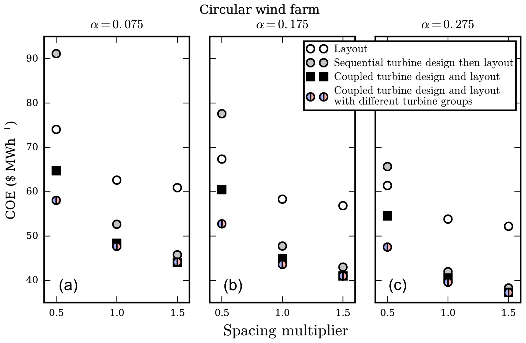
Figure 9The optimal COE results for the circular wind farm layout with 32 turbines. Each of the subfigures corresponds to optimization runs with a different shear exponent, α=0.075, 0.175, and 0.275. Within each subfigure, the x axis shows the size of the wind farm based on the spacing multiplier β=0.5, 1.0, and 1.5. The different points represent the layout optimization with the baseline turbine design, sequential optimization of turbine design and then layout, coupled-layout-and-turbine-design optimization with homogeneous turbine design throughout the farm, and layout-and-turbine-design optimization with two different turbine design groups.

Download

3.1.1 Circular wind farm: sequential optimization of turbine design, then layout

The gray dots in Fig. 9 show the optimal COE results for a sequential optimization. First, a turbine was designed for minimal COE in isolation with the free-stream wind conditions. This turbine design was then used in a wind farm where the layout was subsequently optimized. The rotor diameter was constrained such that the turbine spacing constraints would be satisfied in the baseline farm where the turbine would be installed. This was only applicable for the smallest wind farms, where β=0.5. For each shear exponent, the optimal turbine design was the maximum rotor diameter and turbine rating allowed by the optimizer. The rotor diameter was constrained by the spacing constraint for β=0.5 and by the bound constraint for other turbine spacings. Figure 10 shows the optimal isolated turbine designs for each shear exponent and spacing multiplier, as well as the baseline turbine design. Because these turbines are optimized in isolation and the spacing constraint was not active, the designs for $\mathit{\beta }=\mathrm{1.0},\mathrm{1.5}$ are the same. When these optimized turbine designs are used in each wind farm instead of the baseline turbine design, there is a large COE improvement for the spacing multipliers of β=1.0, 1.5. For β=1.0, COE decreases 15.9 %–22.0 % compared to an optimized wind farm with the baseline turbine design. For β=1.5 the COE decrease is even larger: 24.8 %–26.6 % across all shear exponents. For the smallest wind farm, β=0.5, the turbine design optimized in isolation results in an extremely inefficient wind farm. When in the wind farm environment, exposed to much lower average wind speeds, this design results in a COE that is much worse than the baseline turbine design. The expense from a bigger and taller turbine, coupled with the strong wake interactions among turbines that are so closely spaced means that for this wind farm, optimizing the turbine in isolation actually decreases the wind farm performance.

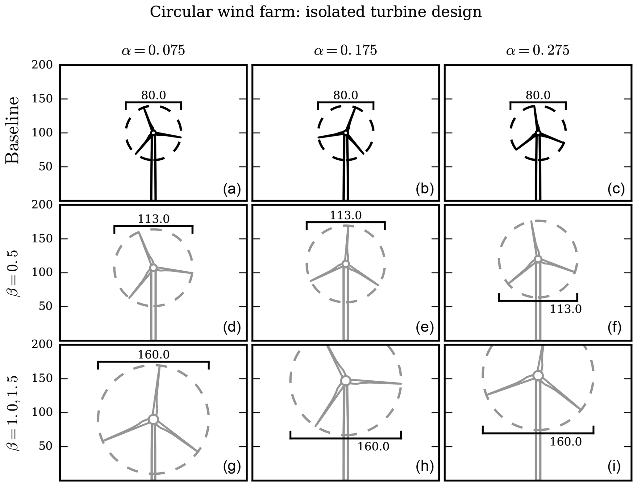
Figure 10The optimal turbine heights and rotor diameters for the isolated turbine design optimization for the circular farm wind conditions. These designs were then used in the sequential optimizations of turbine design, then layout. The columns, from left to right, show the turbines optimized for α=0.075, 0.175, and 0.275. The rows, from top to bottom, show the baseline turbine design, the turbine optimized for the small wind farm (β=0.5), and the turbine designs for the larger wind farms (β=1.0, 1.5).

Download

3.1.2 Circular wind farm: coupled turbine-design-and-layout optimization

Next we will discuss the optimization results of the coupled turbine-design-and-layout optimizations, represented by the black squares in Fig. 9. For every shear exponent and spacing multiplier, there is a large benefit to performing the coupled turbine-design-and-layout optimization compared to the layout-only optimization with the baseline turbine design. Additionally, and more importantly, the coupled optimization results in an appreciably lower COE than the sequential design-then-layout optimization. Obviously for a spacing multiplier of β=0.5, the coupled optimization is far superior to the sequential one simply by being better than the baseline turbine design. For the spacing multiplier of β=1.0, compared to the sequential optimizations, coupled optimization results in an additional 6.82 %, 4.75 %, and 2.65 % COE improvement from layout-only optimization for shear exponents α=0.075, 0.175, and 0.275, respectively. For the largest wind farm, β=1.5, the coupled optimization results in an additional 2.78 %, 3.50 %, and 1.88 % COE improvement compared to the sequential case.

Figure 11The optimal turbine heights and rotor diameters for the optimization runs with coupled layout and turbine design with homogeneous turbine design throughout the circular wind farm. Each column shows a different shear exponent, with α=0.075, 0.175, and 0.275 from left to right. Each row shows a different farm spacing multiplier, with β=0.5, 1.0, and 1.5 from top to bottom.

Download

There are several conclusions we can draw from both the sequential and coupled turbine design and layout optimizations. First, and most apparent, optimizing turbine design results in a much better wind farm than a farm in which the turbines are selected arbitrarily or a priori. Second, and more importantly, optimizing turbine design coupled with the turbine layout is significantly better than optimizing the turbine design for the free-stream wind conditions alone. In a wind farm, turbines rarely experience the free-stream wind conditions as they are often waked by the other turbines in the farm. Therefore, the optimal turbine design is based on on average slower wind speeds than the free-stream wind. This results in turbines with smaller hub heights, rotor diameters, and rated powers. One could conceivably optimize the turbine design for some wind speed slower than the free stream and closer to the average speed in the wind farm, which would likely be better than optimizing the turbine design for the free-stream wind speed. However, the average wind speed in a farm is dependent on the turbine layout, making it difficult to choose the correct speed for which to design the turbines. Thus, is important to couple the turbine design and layout optimization for a superior wind farm.

Figure 11 shows the optimal rotor diameters and hub heights for the coupled turbine-design-and-layout optimizations. For a spacing multiplier β=0.5, the turbines are very close together and in general are heavily waked. Thus to satisfy spacing constraints and because the average wind speed is very low, the optimal rotor diameter is small: about 90 m. When the turbines are spaced farther apart, shown for the larger spacing multipliers, the optimal rotor diameter is much larger: closer to 120–130 m. In these farms, wake interactions are not as severe, meaning that the extra power production from larger rotors is worth the extra turbine capital cost. Also notice the trend of the optimal turbine height with wind shear exponent: for a low wind shear exponent, α=0.075, the wind speed does not drastically change with height (see Fig. 7). Therefore, for this wind condition it is desirable to have short hub heights with a lower turbine capital cost. For the higher shear exponents, $\mathit{\alpha }=\mathrm{0.175},\mathrm{0.275}$, the wind speed increases much more with height (See Fig. 7). In these cases, for every spacing multiplier, the extra cost of building the taller turbines is made up for in the additional power produced from the high wind speeds. Remember that a larger rotor diameter reduces the relative spacing between turbines in the farm, as the original spacing was based on a diameter of 80 m.

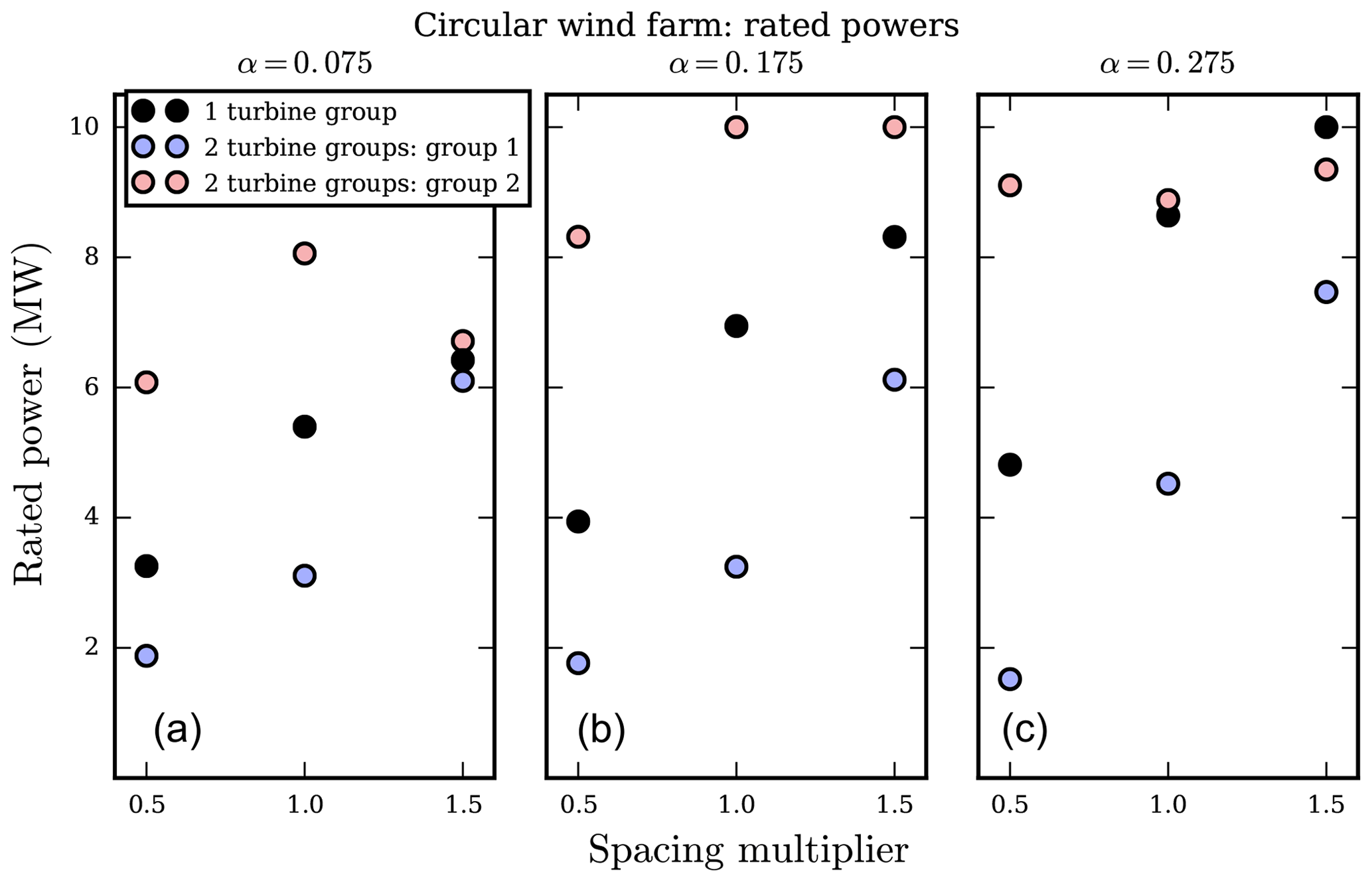
Figure 12The optimal rated powers for the circular wind farm for the optimization runs with coupled layout and turbine design for both uniform wind farm turbine design and with two different turbine design groups. The three subfigures show a different shear exponent, with α=0.075, 0.175, and 0.275 from (a) to (c). Within each subfigure, the x axis shows different farm spacing multipliers, with β=0.5, 1.0, and 1.5.

Download

In Fig. 12, the black points show the optimal rated powers for the turbines in each optimization case. The optimal rated power scales with the turbine rotor diameter and hub height. Higher turbine rating is expensive; therefore, the small rotors and short turbines, which are more heavily waked and do not produce as much power, do not require a large power rating. The extra cost is not justified by a very slight increase in power. For the high shear exponents and spacing multipliers, the turbines are exposed to faster wind speeds. These turbines are bigger and taller, and the extra power production from raising the rated power is worth the additional cost.

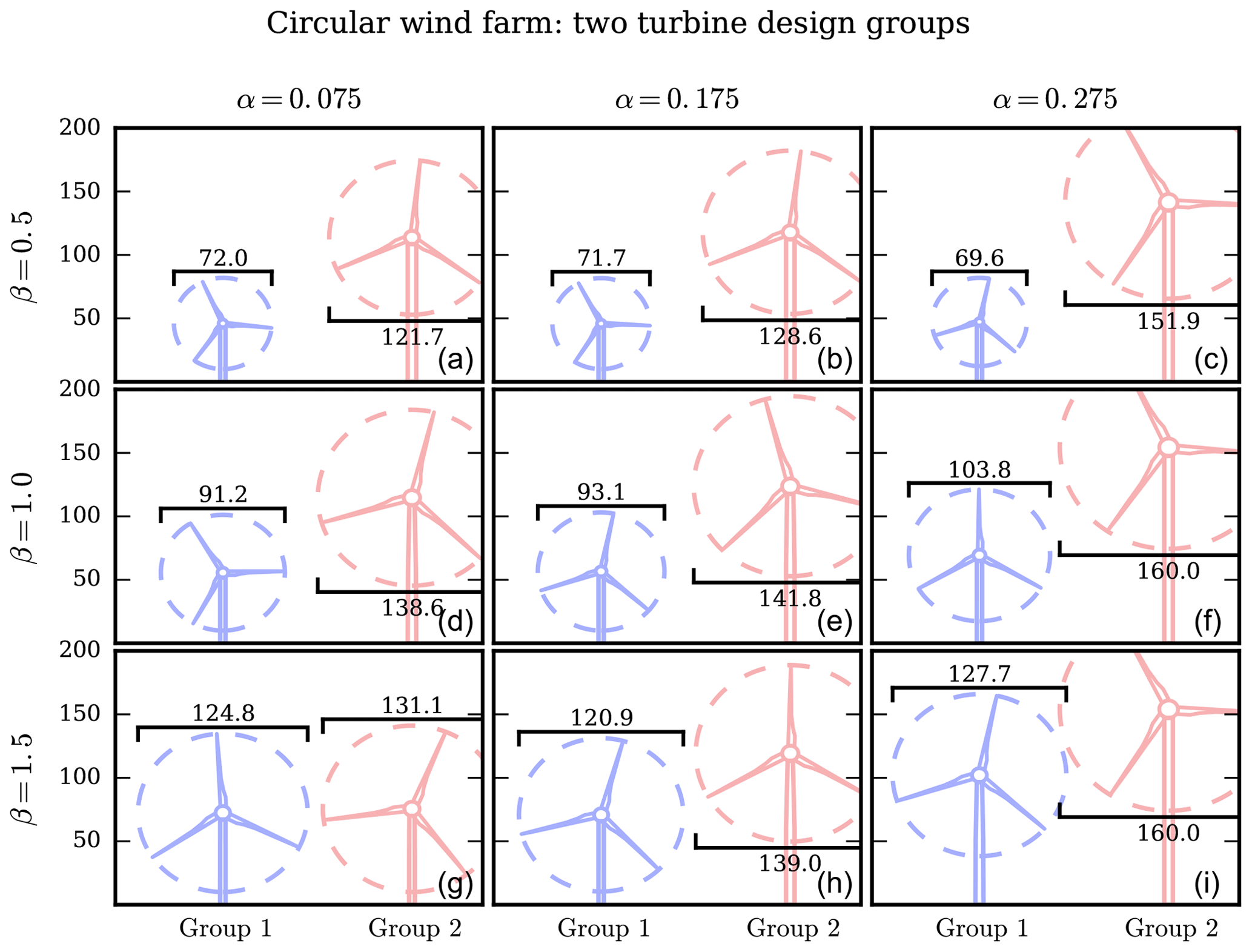
Figure 13The optimal turbine heights and rotor diameters for the optimization runs with coupled layout and turbine design with two different turbine design groups for the circular wind farm. Each column shows a different shear exponent, with α=0.075, 0.175, and 0.275 from left to right. Each row shows a different farm spacing multiplier, with β=0.5, 1.0, and 1.5 from top to bottom.

Download

3.1.3 Circular wind farm: coupled turbine-design-and-layout optimization with two turbine groups

Now we will discuss the most interesting case, the coupled turbine-design-and-layout optimization with two different turbine groups. The optimal COE results of these optimizations are shown by the blue and pink points in Fig. 9. Most visibly, for the smallest spacing multiplier, β=0.5, there is a large COE improvement for the heterogeneous turbine design optimizations compared to the farms with homogeneous turbine design (shown by the black squares in Fig. 9). For this spacing multiplier, the heterogeneous turbine design farms reduce COE by 21.6 %, 21.67 %, and 22.6 % compared to the layout-only optimization for shear exponents of α=0.075, 0.175, and 0.275, respectively. The coupled optimizations with one turbine group reduce COE by 12.59 %, 10.24 %, and 11.15 %. For the smallest spacing multiplier, optimizing turbine design and layout with two turbine groups reduces COE by an additional 9 %–11.45 % compared to just one turbine group. For the spacing multiplier β=1.0, the coupled optimization with two turbine groups results in an additional 1.16 %–2.35 % COE decrease compared to with one turbine group. This is much smaller than the more tightly packed wind farms but still non-negligible. For the spacing multiplier β=1.5, the optimization with two turbine groups results in only an additional 0 %–0.12 % COE decrease, indicating that when the turbines are spread very far apart, there is no benefit to allowing multiple turbine designs in the same farm.

The two different rotor designs in the same wind farm help to improve COE by reducing the wake interaction between wind turbines. By combining tall and short turbines, with large and small rotor sizes, there are more dimensions that the optimizer can manipulate to avoid wakes and improve performance. For the tightly packed wind farms, the turbine layout is greatly limited by the turbine spacing constraints. Additionally, as the turbines are closer together, the wakes greatly reduce the wind speed as they have not had an opportunity to mix with the free-stream air. Both of these factors mean there is a large benefit to avoiding the wakes of other turbines by any means possible. For the larger wind farms where the turbines are spaced farther apart, the wakes are not as detrimental and there is more area in which to avoid wakes in the horizontal plane without needing to change hub height or rotor diameter. In these cases, the heterogeneous turbine designs are not as beneficial.

Figure 13 shows the optimal rotor diameter and hub height of each turbine group for these cases of coupled turbine design and layout optimization with two different groups. For the spacing multiplier β=0.5, when the turbines are very close together, there is a large difference in both the rotor diameter and hub height of each turbine group. Group 1 is extremely small and short, smaller than even the baseline rotor diameter, while group 2 is much larger. Even if turbines from each group were immediately adjacent to each other, there would be minimal wake interaction between the turbines. For the small wind farms, the sacrifice in power that comes from one very small and short turbine is made up for in the decreased wake interference between turbine groups. Essentially, having two different turbine groups doubles the effective spacing between turbines because turbines in different groups do not affect each other. For a larger spacing multiplier of β=1.0, each turbine group is still remarkably different in size and height. The turbines are larger than they were for the smallest wind farm because the average wind speed is faster when the turbines are spread farther apart. Notice that, compared to the optimized turbines for β=0.5, the smaller turbines when β=1.0 are larger and overlap more with the taller, bigger turbines. In this case, the power increase from bigger rotor diameters outweighs the benefit gained from reducing wake interference.

The turbine sizes for the largest wind farm, β=1.5, demonstrate the multimodality of the wind farm optimization problem. For this spacing multiplier, each turbine group is more similar than in the previous wind farm sizes. For the lowest shear exponent, α=0.075, both turbine groups are almost identical. For α=0.175, 0.275, there is some difference in each rotor diameter and hub height, although the difference is not as pronounced as it was for the smaller wind farms. However, Fig. 9 shows that for β=1.5 the optimal COE from coupled turbine-design-and-layout optimization is almost exactly the same with one and two turbine groups. So, a wind farm with the homogeneous turbine design shown in the bottom row of Fig. 11 and a wind farm with two different turbine designs shown in the bottom row of Fig. 13 result in a very similar optimal COE. The same optimal result is achieved with drastically different farms, each with different turbines and layouts.

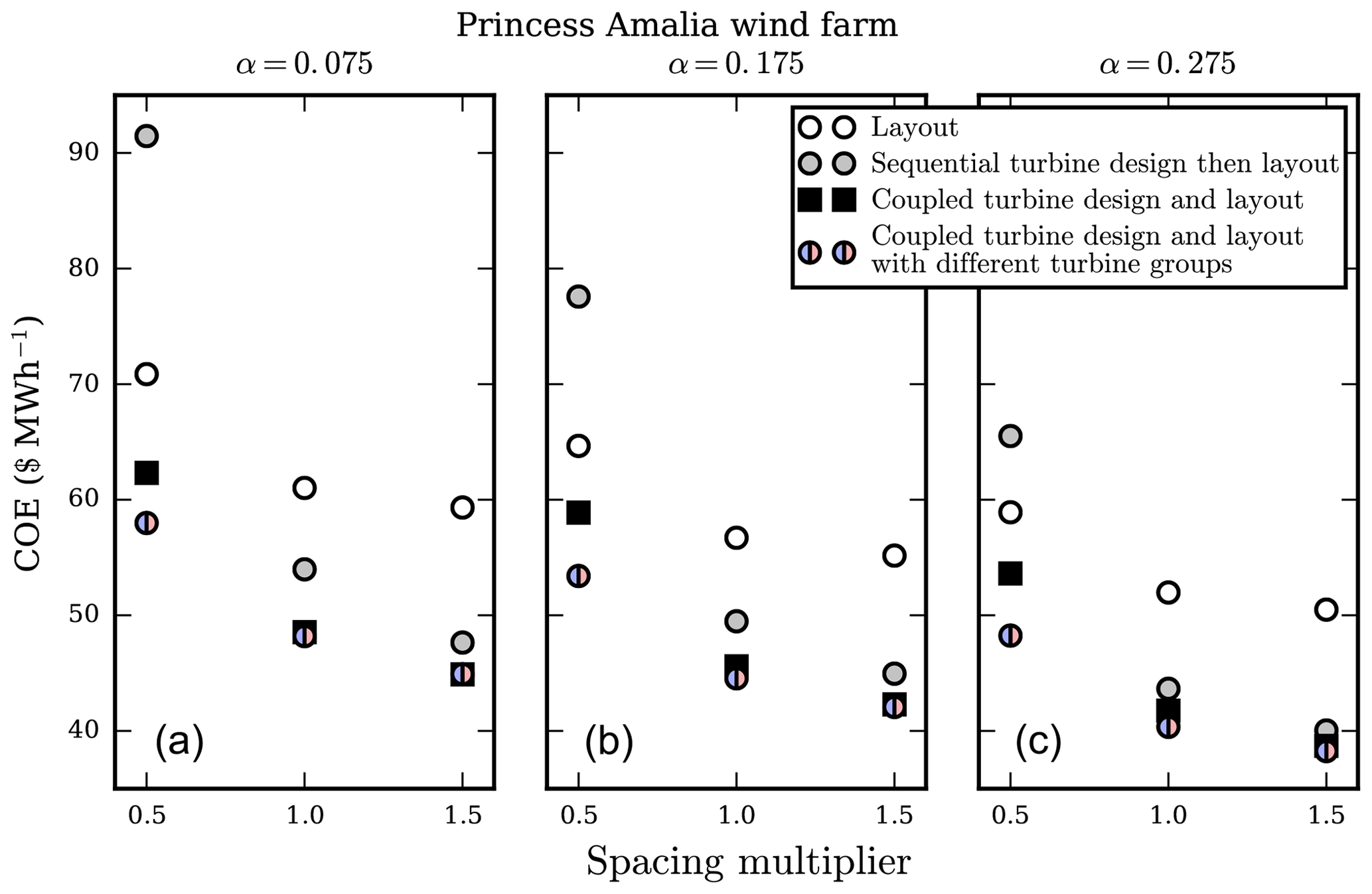
Figure 14The optimal COE results for the Princess Amalia wind farm layout with 60 turbines. Each of the subfigures corresponds to optimization runs with a different shear exponent, from (a) to (c) α=0.075, 0.175, and 0.275. Within each subfigure, the x axis shows the size of the wind farm based on the spacing multiplier, β=0.5, 1.0, and 1.5. The different points represent the layout optimization, sequential optimization of turbine design and then layout, coupled layout-and-turbine-design optimization with homogeneous turbine design throughout the farm, and layout-and-turbine-design optimization with two different turbine design groups.

Download

Figure 12 shows the optimal rated power of each height group for the optimization cases with two different turbine groups. The blue and pink dots in this plot correspond to the turbines of the same color in Fig. 13. As with the homogeneous turbine wind farm, the optimal rated power scales with the optimal turbine height and diameter. These larger, taller turbines are optimal in wind farms where they will be exposed to high wind speeds and produce large amounts of power. From a power production standpoint, it is undesirable to ever have a turbine's power limited by the rating. However, turbines with high ratings are more expensive and not worth the cost if the turbine is generally producing low amounts of power. Therefore, the short, small turbines are optimal with a low, cheap power rating. The larger, taller turbines, which produce much more electricity, utilize the higher ratings.

3.2 Princess Amalia wind farm results

In this section, we will discuss the results from the Princess Amalia wind farm optimizations. All of the optimizations that were performed with the circular, 32-turbine wind farm were repeated for the larger, 60-turbine Princess Amalia wind farm. We will show and briefly discuss the optimal COE results; however, the optimal turbine designs for the Princess Amalia wind farm optimizations were very similar to those for the circular wind farm and therefore will not be included in this paper.

Figure 14 shows the COE results for the 60-turbine Princess Amalia wind farm optimizations. The trends are similar to the smaller, circular wind farm. Coupled turbine design and layout optimization is superior to optimizing each sequentially, especially for the smaller wind farms where the wind speeds are much lower than the free stream. For the farms with closely spaced wind turbines, two different turbine designs in the same farm are significantly better than the farms optimized with a homogeneous turbine design. If the largest wind farms (β=1.5) benefit from two different turbine design groups, that benefit is negligible. The optimal COE values for the Princess Amalia wind farm are slightly lower across the board than the circular wind farm COE values. This is partly because there are more turbines in the Princess Amalia wind farm so a smaller portion of the total cost comes from overhead but also is partly due to the Princess Amalia wind turbines being spaced slightly farther apart than those in the circular wind farms. Another major difference between the optimal COE values of each wind farm is in the optimization case with two turbine design groups. For the Princess Amalia wind farm and a spacing multiplier of 0.5, two turbine groups provide an additional COE decrease of 6.13 %–9.11 % compared to the wind farm with homogeneous turbine design. This is significant; however, it is not as large as the 9.01 %–11.45 % additional COE decrease in the circular wind farm optimizations for the same spacing multiplier. Again, the main cause of this seems to be that the turbines in the circular wind farms are slightly closer together than the turbines in the Princess Amalia wind farms.

Table 1The percent COE decrease in the various optimization cases with respect to layout-only optimization. This table does not show the overall desirability of the optimal wind farm but the relative improvement of different considerations of turbine design optimization. In the table are shown results for each shear exponent, α, as well as each spacing multiplier, β, in which the smaller spacing multipliers represent farms with turbines that are more closely spaced. Bold entries performed worse than the baseline layout-only optimization.

Download Print Version | Download XLSX

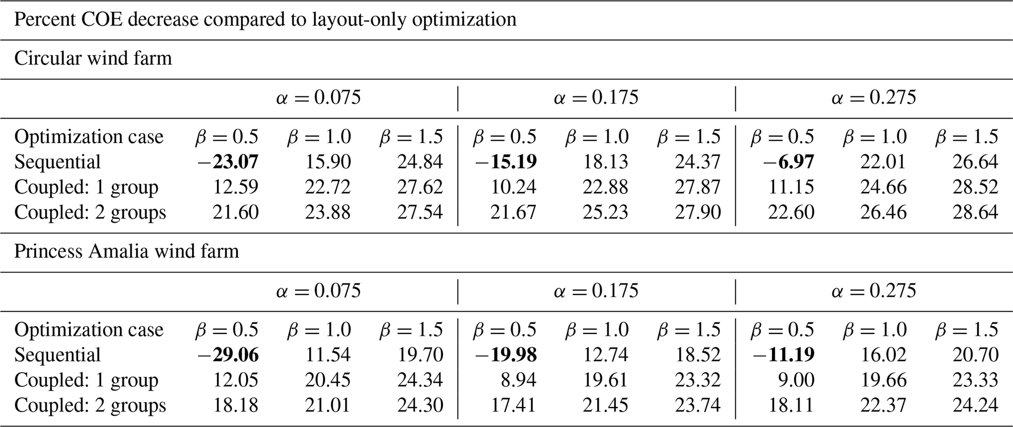
Table 1 shows how the optimal COE results for each wind farm compared to the layout optimization with the baseline wind turbine design. These numbers compare the relative benefit of performing turbine design with the various scenarios mentioned. High numbers represent a large COE decrease compared to the layout-only optimization for a given shear exponent and spacing multiplier combination; they do not necessarily represent a low COE. There are a few interesting numbers in this table. Most obvious are the negative values (shown in bold) for the sequential optimization with a spacing multiplier of 0.5. For these farms, sequential optimization is actually worse than the baseline. Also notice the COE decrease from coupled optimization with one group to two groups. For β=0.5, there is a huge benefit to having two groups, for β=1.0 there is a small benefit, and for β=1.5 there is no benefit at all. Finally, the benefit of coupled optimization with one group compared to sequential optimization is important. Again, there is a huge benefit to coupled optimization for the smallest spacing multiplier, and this relative benefit decreases as the wind farm size grows. However, even for β=1.5, there is an appreciable benefit to coupled design-and-layout optimization compared to sequential optimization.