2.1 Aerodynamics

The theory underlying this Aerodynamics section is found in Sørensen (2016).

For wind turbine aerodynamics non-dimensional coefficients are often introduced and some of the common ones are for the rotor thrust (C_T) and power (C_P).

where T and P are the rotor thrust and power, respectively; ρ is the air density, V is the undisturbed flow speed and R is the rotor radius.

These definitions can be applied for any wind turbine rotor, but in this paper, we will use a simplified relationship between C_T and C_P that is derived from classical 1-D momentum theory. This implies an assumption of uniform aerodynamic loading across the rotor plane. The classical equations are often given in terms of the axial induction (a), which is defined as $a=\mathrm{1}-\frac{V_{\mathrm{rotor}}}{V}$, where V_rotor is the axial flow speed in the rotor plane. By combining the two classical momentum theory expressions for C_P(a) and C_T(a) (Sørensen, 2016, p. 11, Eq. 3.8), the relationship between these coefficients is arrived at as follows:

where a(C_T) is found by inverting C_T(a) and using the negative solution. A plot of C_T vs. C_P can be seen in Fig. 1. This C_P(C_T) curve is monotonically decreasing in slope and reaches a maximum of $C_{\mathrm{P}}=\mathrm{16}/\mathrm{27}$, corresponding to the well-known Betz limit at $C_{\mathrm{T}}=\mathrm{8}/\mathrm{9}$. These monotonicity properties lead to the key observation that a reduction in thrust ($C_{\mathrm{T}}=\mathrm{8}/\mathrm{9}-\mathrm{\Delta }{C}_{\mathrm{T}}$) will not lead to a proportional change in power (ΔC_P). This motivates the investigation in this paper of the trade-off between power and loads.

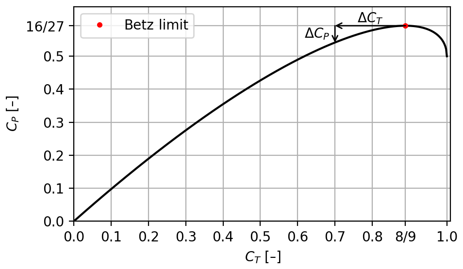
Figure 1Relationship between normalized rotor load C_T and power coefficient C_P from 1-dimensional momentum theory. Note that around the Betz limit a small change in C_T does not lead to a proportional change in C_P; this is illustrated by ΔC_T and ΔC_P.

Download

2.1.2 Baseline rotor

The work here aims to demonstrate an improved rotor performance compared to a baseline design. This baseline design is chosen to be a turbine operating at the Betz limit below the rated wind speed and keeping a constant power above the rated power.

$$\begin{array}{}\text{(8)}& C_{\mathrm{T},\mathrm{0}}={\displaystyle \frac{\mathrm{8}}{\mathrm{9}}}\approx \mathrm{0.889};C_{\mathrm{P},\mathrm{0}}={\displaystyle \frac{\mathrm{16}}{\mathrm{27}}}\approx \mathrm{0.593}\end{array}$$

This choice of baseline mimics the typical practice of designing wind turbines target operation at the maximum C_P below the rated power. In reality, turbines will not achieve a maximum C_P at $C_{\mathrm{T}}=\mathrm{8}/\mathrm{9}$ since losses alter the relationship between C_T and C_P, but this does not change the fact that turbines are operated at the point of the maximum C_P. Figure 2 shows the power and thrust curves for the baseline rotor.

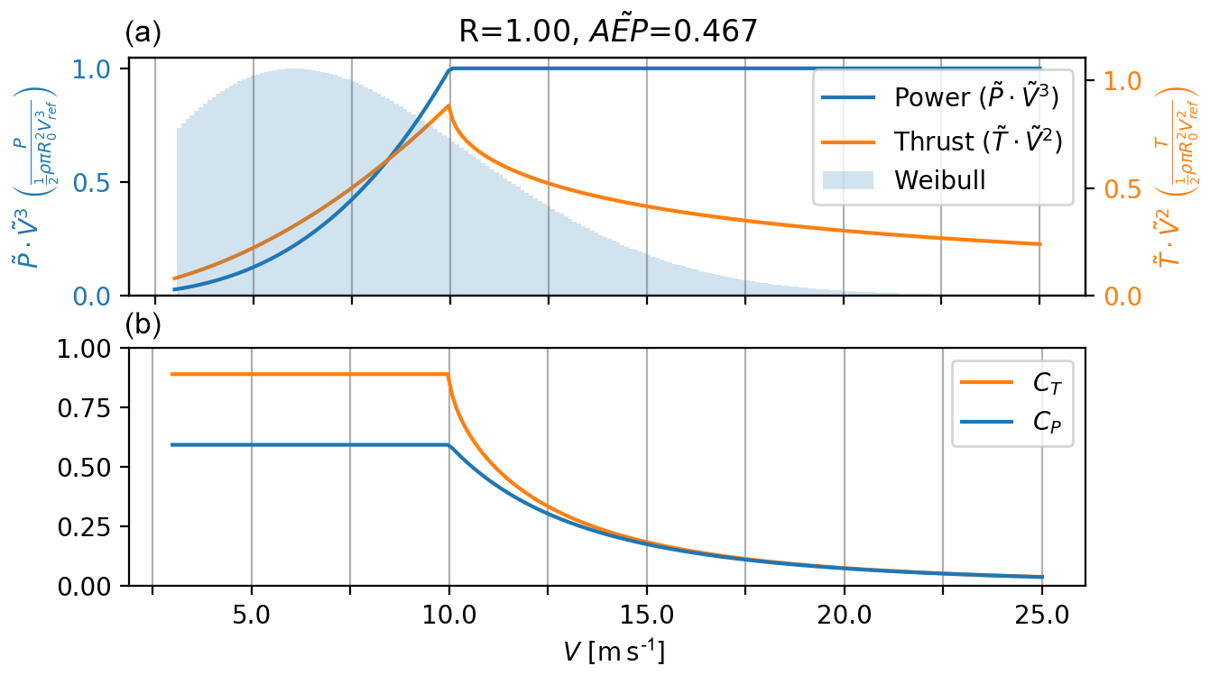
Figure 2(a) The dimensionless power and thrust for the baseline rotor as a function of wind speed. Overlaid (in blue) is the Weibull wind speed frequency distribution used throughout (IEC-class III: V_avg=7.5; k=2). (b) C_T and C_P as a functions of wind speed. These curves reflect how most turbines are operated today, targeting the maximum power coefficient below the rated power, which leads to a thrust peak just before the rated power.

Download

In this paper, all results are presented as the change in performance relative to that of the baseline rotor. For this reason, all of the relevant variables (denoted with a zero in the subscript) will be normalized by the corresponding baseline rotor values.

$$\begin{array}{}\text{(9)}& {\displaystyle }& {\displaystyle }\mathrm{\Delta }R={\displaystyle \frac{R}{R_{\mathrm{0}}}}-\mathrm{1}\text{(10)}& {\displaystyle }& {\displaystyle }\mathrm{\Delta }\stackrel{\mathrm{̃}}{P}={\displaystyle \frac{C_{\mathrm{P}}{R}^{\mathrm{2}}}{C_{\mathrm{P},\mathrm{0}}{R}_{\mathrm{0}}^{\mathrm{2}}}}-\mathrm{1}\text{(11)}& {\displaystyle }& {\displaystyle }\mathrm{\Delta }\stackrel{\mathrm{̃}}{L}={\displaystyle \frac{C_{\mathrm{T}}{R}^{L_{\exp }}}{C_{\mathrm{T},\mathrm{0}}{R}_{\mathrm{0}}^{L_{\exp }}}}-\mathrm{1}\text{(12)}& {\displaystyle }& {\displaystyle }\mathrm{\Delta }\stackrel{\mathrm{̃}}{\mathrm{AEP}}={\displaystyle \frac{\stackrel{\mathrm{̃}}{\mathrm{AEP}}}{{\stackrel{\mathrm{̃}}{\mathrm{AEP}}}_{\mathrm{0}}}}-\mathrm{1},\end{array}$$

where $\stackrel{\mathrm{̃}}{L}$ as well as L_exp is a generalized load that is introduced in Sect. 4.1 (Effects on loads), and it is written here for later reference.

2.2 Scale laws and constraints for design-driving loads

In this section, examples of static aerodynamic design-driving loads (DDLs) will be presented. These examples are not meant to be exhaustive but include several of the key considerations that constrain the practical design of wind turbine rotors. From the scaled loads, design-driving load constraints (DDLCs) are introduced, which limit loads so that these do not exceed the levels of the baseline rotor. Based on the DDL examples, it is shown that DDLCs can be elegantly put in a generalized form.

2.2.4 Tip deflection with constant mass

The final example of a DDL is also based on tip deflection but includes a condition to maintain a constant mass of the load-carrying structure of the blade. To this end, the stylized spar-cap layout depicted in Fig. 3 is assumed. This layout consists of two planks. The stiffness of a spar-cap structure with a homogeneous Young's modulus (E) can be found from the stiffness of the rectangle and the parallel axis theorem (see Fig. 3 for the variable definitions) as follows:

$$\begin{array}{}\text{(24)}& \begin{array}{rl}& \left.\begin{array}{l}{I}_{\mathrm{rect}}=\frac{B{h}^{\mathrm{3}}}{\mathrm{12}}\\ EI=\mathrm{2}E\left(I_{\mathrm{rect}}+A{\left(\frac{H-h}{\mathrm{2}}\right)}^{\mathrm{2}}\right)\\ A=Bh\end{array}\right\}\\ & EI=\mathrm{2}E\left({\displaystyle \frac{B{h}^{\mathrm{3}}}{\mathrm{12}}}+Bh{\left({\displaystyle \frac{H-h}{\mathrm{2}}}\right)}^{\mathrm{2}}\right)\\ & =E{\displaystyle \frac{H^{\mathrm{2}}Bh}{\mathrm{2}}}\left({\displaystyle \frac{h^{\mathrm{2}}}{\mathrm{3}{H}^{\mathrm{2}}}}+{\left(\mathrm{1}-{\displaystyle \frac{h}{H}}\right)}^{\mathrm{2}}\right).\end{array}\end{array}$$

For modern wind turbines $h/H\ll \mathrm{1}$, meaning that a common approximation is

$$\begin{array}{}\text{(25)}& EI\approx E{\displaystyle \frac{H^{\mathrm{2}}Bh}{\mathrm{2}}}.\end{array}$$

To compute the mass for such a structure it will be assumed that plank height h and the plank width B are constant and the change in EI comes from a decrease in building height H. Then, if h is decreased when R is increased, the following relationship needs to be satisfied for the mass of the planks to be constant (assuming a constant mass density),

$$\begin{array}{}\text{(26)}& Rh=R_{\mathrm{0}}{h}_{\mathrm{0}}.\end{array}$$

From there it follows that changes in the radius of the rotor will change the stiffness as

$$\begin{array}{}\text{(27)}& \left.\begin{array}{l}EI\approx E\frac{H^{\mathrm{2}}Bh}{\mathrm{2}}\left(\mathrm{25}\right)\\ h=\frac{R_{\mathrm{0}}{h}_{\mathrm{0}}}{R}\left(\mathrm{26}\right)\end{array}\right\}EI\approx E{\displaystyle \frac{H^{\mathrm{2}}B{R}_{\mathrm{0}}{h}_{\mathrm{0}}}{\mathrm{2}R}}.\end{array}$$

Combining this equation with the tip deflection equation (Eq. 21), scaling and DDLC can be found as follows:

$$\begin{array}{}\text{(28)}& \begin{array}{rl}& \begin{array}{l}\mathrm{Scaling}\\ \left.\begin{array}{l}{\mathit{\delta }}_{\mathrm{tip}}=\frac{\mathrm{11}\mathit{\pi }}{\mathrm{120}}\frac{V^{\mathrm{2}}\mathit{\rho }}{E{I}_{\mathrm{r}}}{C}_{\mathrm{T}}{R}^{\mathrm{5}}{\mathit{\delta }}_{\mathrm{shape}}\left(\stackrel{\mathrm{̃}}{r}=\mathrm{1},\frac{E{I}_{\mathrm{r}}}{E{I}_{\mathrm{t}}}\right)\\ EI\approx E\frac{H^{\mathrm{2}}B{R}_{\mathrm{0}}{h}_{\mathrm{0}}}{\mathrm{2}R}\end{array}\right\}\end{array}\\ & \Rightarrow \begin{array}{l}\mathrm{DDLC}\\ \left({\mathit{\delta }}_{\mathrm{tip}+\mathrm{mass}}\right)=\frac{C_{\mathrm{T}}}{C_{\mathrm{T},\mathrm{0}}}\frac{E{I}_{\mathrm{r},\mathrm{0}}}{E{I}_{\mathrm{r}}}{\left(\frac{R}{R_{\mathrm{0}}}\right)}^{\mathrm{5}}=\frac{C_{\mathrm{T}}}{C_{\mathrm{T},\mathrm{0}}}{\left(\frac{R}{R_{\mathrm{0}}}\right)}^{\mathrm{6}}\le \mathrm{1},\end{array}\end{array}\end{array}$$

with the use of the fact that changing h by the same magnitude for the whole blade leads to $\frac{E{I}_{\mathrm{r}}}{E{I}_{\mathrm{t}}}=\frac{E{I}_{\mathrm{r},\mathrm{0}}}{E{I}_{\mathrm{t},\mathrm{0}}}$ and thereby does not affect δ_shape. It should be noted that choosing B to change instead will lead to the same scaling but the difference is that changing the plank thickness might lead to higher-order effects, although they are expected to be insignificant.

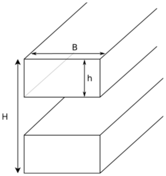
Figure 3Assumed spar-cap structure with dimensions: H is the total build height, h is the space between planks and B is the plank width.

Download

3.1 Power-capture optimization

The optimization problem can be stated as

where the definition of $\stackrel{\mathrm{̃}}{R}=R/R_{\mathrm{0}}$ has been used for consistency. The solution for this optimization problem is presented in Sect. 4.1.

It should be noted that this optimization problem is similar to the problem that is given by Chaviaropoulos and Sieros (2014) in which they optimize while keeping M_flap. So the optimization problem in this paper is a generalization of their optimization problem.

3.2 AEP optimization

In contrast to the above mentioned optimization of power capture, optimization with respect to AEP requires the determination of $C_{\mathrm{T}}\left(\stackrel{\mathrm{̃}}{V}\right)$, so it involves a function opposed to a scalar value. It is also necessary to set the rated power to constant value, while the wind speed at which the rated power is reached is allowed to change. The problem can be formulated as

where the wind speed scaling has been added to the DDLC.

4.1 Optimizing for power capture

The constrained optimization problem maximizing power capture, as stated in Sect. 3, may be simplified based on the observation that optimum solutions will occur at the DDL constraint limit. To understand this, consider that the power capture of a rotor with an inactive constraint may always be improved by scaling the rotor up until the constraint is met. This is true irrespective of the DDLC that determines the rotor design. Hence, an explicit relation $\stackrel{\mathrm{̃}}{R}\left(C_{\mathrm{T}}\right)$ can be used to reformulate the problem from a constrained optimization problem in two variables to an unconstrained optimization problem in one variable.

with the optimization problem now as follows:

By differentiating the objective function (Eq. 35 with respect to C_T and finding its root, the optimal C_T as a function of R_exp is arrived at.

This unique solution is a maximum, which is apparent from the always-positive value of ΔP in Fig. 4. This figure shows the optimal solution for C_T and C_P, as well as the relative change in radius (ΔR) and power (ΔP) compared to the baseline rotor. In the plots in Fig. 4a and c, C_P is observed to approach the dashed baseline performance (Betz rotor) much faster than C_T as R_exp increases. This is a consequence of the relationship between C_T and C_P (Fig. 1). Especially around the Betz limit, the gradient is very small, which means that changes in C_T do not lead to proportional changes in C_P. Turning to the two plots in Fig. 4b and d, it is seen that the lower C_P is more than compensated for by increasing R since the relative change in power (ΔP) is always positive.

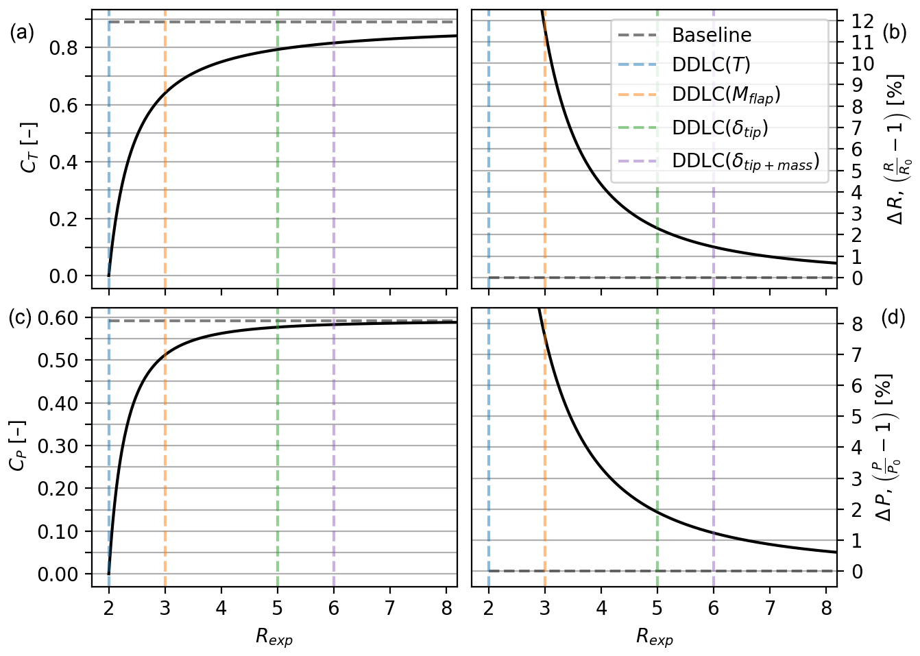
Figure 4(a) Optimal C_T as a function of the constraint R exponent (R_exp). (c) R_exp vs. C_P; notice that the optimal C_P curve has a steeper slope and hugs the baseline closer than C_T. (b) R_exp vs. relative change in radius ΔR. (d) R_exp vs. relative change in power capture ($\mathrm{\Delta }\stackrel{\mathrm{̃}}{P}$). Despite the similar shape of the curves, a difference between the two is that $\mathrm{\Delta }P(R_{\exp }\to \mathrm{2})=\mathrm{50}$ %, while $\mathrm{\Delta }R(R_{\exp }\to \mathrm{2})\to \mathrm{\infty }$. The vertical lines represent each of the example constraints (^* DDLC: design-driving load constraint).

Download

When maximizing power capture for a given thrust (R_exp=2; dashed vertical blue line in Fig. 4), it is found that C_T→0 and ΔR→∞ while ΔP→50 %, which was found by investigating the behavior of the limit value when R_exp→2. Since ΔR→∞ is not of much practical interest, further explanation is not given here. Alternatively, the maximum power for a given flap root moment (R_exp=3; orange line in Fig. 4) may be achieved by increasing the rotor radius by 11.6 % compared to the baseline design (maximum C_P). The corresponding relative increase in power ΔP is 7.6 %. Finally, designs constrained by tip deflection (R_exp=5; green line in Fig. 4) allow the relative power ΔP to increase by 1.90 % with a relative change in radius ΔR of 2.30 %. A table with the results for the increase in power capture (ΔP) and radius (ΔR) for four designs (R_exp=2, 3, 5, 6) can be seen in Fig. 6. In conclusion, rotors with a static aerodynamic DDLC should not be designed for the maximum C_P, as more power can be generated by rotors with a lower C_T and a larger radius R, without violating the relevant DDLC.

Effect on loads

Even though meeting the constraint limits means that the chosen DDL will be the same as the baseline, it is interesting to know what happens to loads that scale differently than the DDL. As an example, if the DDLC is M_flap (R_exp=3) it is a given that it will not change relative to the baseline, but it could be interesting to know what happens to T and δ_tip.

To investigate it we will introduce a generalized load (L) as a measure of how a load scale.

$$\begin{array}{}\text{(39)}& L=K_{\mathrm{0}}{V}_{\mathrm{0}}^{\mathrm{2}}{C}_{\mathrm{T}}{R}^{L_{\exp }},\end{array}$$

where K₀ is a scaling constant and L_exp is the generalized load exponent. The generalized load equation can be made non-dimensional with

$$\begin{array}{}\text{(40)}& \stackrel{\mathrm{̃}}{L}={\displaystyle \frac{L}{K_{\mathrm{0}}{V}_{\mathrm{0}}^{\mathrm{2}}{R}_{\mathrm{0}}^{L_{\exp }}}}=C_{\mathrm{T}}{\stackrel{\mathrm{̃}}{R}}^{L_{\exp }}.\end{array}$$

The difference between L_exp and R_exp is that R_exp results in a design, whereas L_exp is a load for a design. Take a design made for tip deflection (R_exp=5) as an example, then L_exp=3 will describe the M_flap load for that design.

An equation for the relative change $\mathrm{\Delta }\stackrel{\mathrm{̃}}{L}$ can be found in terms of the baseline rotor as follows:

$$\begin{array}{}\text{(41)}& \begin{array}{rl}& \left.\begin{array}{l}\stackrel{\mathrm{̃}}{L}=C_{\mathrm{T}}{\stackrel{\mathrm{̃}}{R}}^{L_{\exp }}\left(\mathrm{40}\right)\\ \stackrel{\mathrm{̃}}{R}={\left(\frac{C_{\mathrm{T},\mathrm{0}}}{C_{\mathrm{T}}}\right)}^{\frac{\mathrm{1}}{R_{\exp }}}\left(\mathrm{30}\right)\\ {\stackrel{\mathrm{̃}}{L}}_{\mathrm{0}}=C_{\mathrm{T},\mathrm{0}}{\stackrel{\mathrm{̃}}{R}}_{\mathrm{0}}^{L_{\exp }}=C_{\mathrm{T},\mathrm{0}}\end{array}\right\}\\ & \Rightarrow \mathrm{\Delta }\stackrel{\mathrm{̃}}{L}={\displaystyle \frac{\stackrel{\mathrm{̃}}{L}}{{\stackrel{\mathrm{̃}}{L}}_{\mathrm{0}}}}-\mathrm{1}={\left({\displaystyle \frac{C_{\mathrm{T}}}{C_{\mathrm{T},\mathrm{0}}}}\right)}^{\mathrm{1}-\frac{L_{\exp }}{R_{\exp }}}-\mathrm{1}.\end{array}\end{array}$$

Since it is known that $C_{\mathrm{T}}\le C_{\mathrm{T},\mathrm{0}}$ these conclusions follow:

$$\begin{array}{ll}{\displaystyle }& {\displaystyle }{L}_{\exp }<R_{\exp }\mathrm{The}\mathrm{load}\mathrm{is}\mathrm{lower}\mathrm{than}\mathrm{the}\mathrm{baseline}\mathrm{level}.\\ {\displaystyle }& {\displaystyle }{L}_{\exp }=R_{\exp }\mathrm{The}\mathrm{load}\mathrm{is}\mathrm{identical}\mathrm{to}\mathrm{the}\mathrm{baseline}\mathrm{level}.\\ {\displaystyle }& {\displaystyle }{L}_{\exp }>R_{\exp }\mathrm{The}\mathrm{load}\mathrm{is}\mathrm{larger}\mathrm{than}\mathrm{the}\mathrm{baseline}\mathrm{level}.\end{array}$$

This agrees with Fig. 5, which illustrates the effect of design constraints (DDLCs) on different loads. For example, consider tip deflection (R_exp=5; DDLC(δ_tip); the dashed green line in Fig. 5). Looking at the solid green line (L_exp=5) it is seen that the relative change in L is zero as expected. Now looking at the loads with L_exp<R_exp, namely thrust (L_exp=2) and flap moment (L_exp=3), it is seen that ΔL is lower than the baseline, with $\mathrm{\Delta }T=-\mathrm{6.6}$ % and $\mathrm{\Delta }{M}_{\mathrm{flap}}=-\mathrm{4.4}$ %. But for loads where L_exp>R_exp the loads are increased. If there was a load that scaled like L_exp=6 the load would be increased by $\mathrm{\Delta }{L}_{(L_{\exp }=\mathrm{6})}=+\mathrm{2.3}$ %. Furthermore, Fig. 5 shows that the relative decrease in load is always most pronounced for the thrust (L_exp=2), with the biggest impact occurring around R_exp≈2.5. All of the relative change curves have distinct minima but at the same time are characterized by large plateaus of relatively small change. Another observation is how quickly the curves grow for L_exp>R_exp. Take DDLC(M_flap) as an example; in this case $\mathrm{\Delta }{\mathit{\delta }}_{\mathrm{tip}}=+\mathrm{24.5}$ % and $\mathrm{\Delta }{L}_{(L_{\exp }=\mathrm{6})}=+\mathrm{38.9}$ %. The relative change in loads becomes smaller as R_exp increases. A sketch with a zoomed-in view of the tip and a table with the values can be seen in Fig. 6.

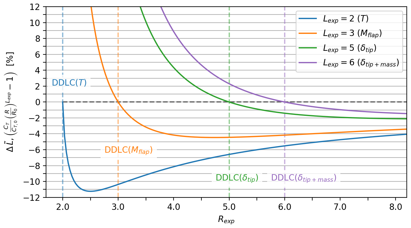
Figure 5Relative change in different rotor load parameters ($\mathrm{\Delta }\stackrel{\mathrm{̃}}{L}$) depending on DDLC. The scaling of loads have the form $\stackrel{\mathrm{̃}}{L}=C_{\mathrm{T}}{R}^{L_{\exp }}$; e.g., L_exp=2 scales as the rotor thrust T and L_exp=5 scales as the tip deflection δ_tip. Each curve depicts how a load parameter would change depending on the design-driving constraint. As an example, consider a design limited by tip deflection DDLC(δ_tip), i.e., R_exp=5, which matches the dashed green line. Tip deflection meets the requirements, while thrust (T) is lowered by 6.6 % and flap moment M_flap by 4.4 %.

Download

Figure 6Sketch of a turbine with the load/structural response outlined. The zoomed-in figure shows the radius increase (ΔR) and the change in tip deflection (Δδ_tip) for two different DDLCs (bold black line is the baseline). The table shows the relative change in power, radius and load/structural response for different DDLCs. R_exp=2 is a thrust constraint design, R_exp=3 is a flap moment constraint design, R_exp=5 is a tip-deflection constraint design and R_exp=6 is the tip deflection+constant mass constraint design.

Download

4.2 Low-induction rotor

The concept in this section was mentioned in the Introduction since it has had some attention over the recent years. The low-induction rotors (LIR) are rotors designed with a lower axial induction a than the level that maximizes C_P. The concept is, to a certain degree, analogous with optimization of rotors for power capture.

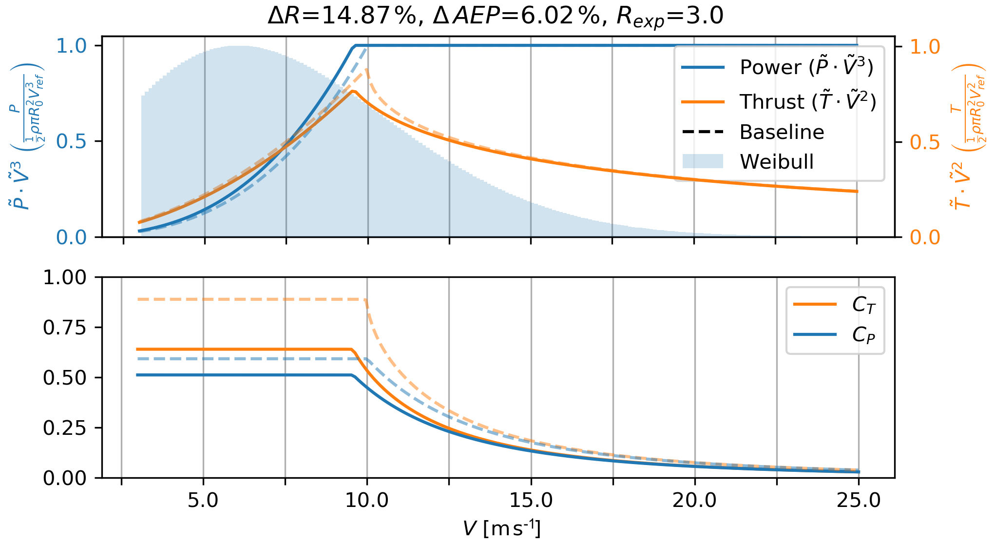
Figure 7Power and thrust curves for a low-induction rotor (solid lines), designed using the present method with the DDLC exponent R_exp=3, which corresponds to an M_flap constraint. The dashed line is the baseline rotor optimized for a max C_P.

Download

To investigate such an LIR design, it was chosen to fix the C_T value below the rated power in order for it to be the same as for the power-capture optimization for a given R_exp. If the radius was set to the same value as for power capture, it will result in the constraint limit not being met since the turbine reaches the rated power earlier. Since C_T is fixed and the constraint limit needs to be met, the wind speed at which the turbine reaches the rated power (${\stackrel{\mathrm{̃}}{V}}_{\mathrm{rated}}$) can be found. It is found through the normalized power (the integrant of Eq. 7 without the PDF_wind) and the constraint limit with wind speed scaling (Eq. 30 multiplied with ${\stackrel{\mathrm{̃}}{V}}^{\mathrm{2}}$) as follows:

For a given rated wind speed the rotor radius can be found using the following steps:

With C_T, ${\stackrel{\mathrm{̃}}{V}}_{\mathrm{rated}}$ and $\stackrel{\mathrm{̃}}{R}$, $\stackrel{\mathrm{̃}}{\mathrm{AEP}}$ can be computed using Eq. (7).

The LIR is illustrated by the examples in Figs. 7 and 8 where the present analysis framework has been applied with constraints pertaining to flap moments (R_exp=3) and tip deflections (R_exp=5).

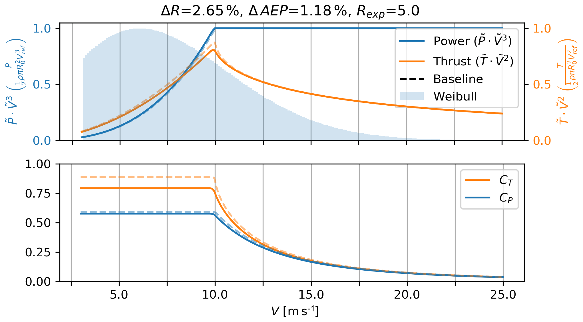
Figure 8Power and thrust curves for rotor with the DDLC exponent R_exp=5 (solid lines), corresponding to a δ_tip constraint. The dashed line is the baseline rotor optimized for max C_P.

Download

In both cases, the resulting power curves are slightly above the equivalent baseline ones, and the thrust peaks are reduced compared to the baseline. The relative change in AEP results in a smaller change than the change in power at the design point. For the case with DDLC(M_flap), ΔAEP=6.0 % while the power capture increased by ΔP=7.6 %. The corresponding improvements for a tip-deflection-constrained rotor, DDLC(δ_tip), are ΔAEP=1.2 % and ΔP=1.9 %. The lower relative improvement for the LIR is related to the amount of the power that is produced below the rated power. The results for the LIR are summarized in Fig. 9 with a table and a sketch showing the relative changes in AEP, radius, thrust, root-flap moment and tip deflection for four different designs (R_exp=2, 3, 5, 6). From Fig. 9 the thrust constraint design (DDLC(T); R_exp=2) is seen to have diverging values for ΔR, ΔM_flap and Δδ_tip. As was the case for power-capture optimization these results are found from investigating the result of the limit in which R_exp→2. Even though the result of ΔR→∞ is interesting, the corresponding consequence of ΔM_flap→∞ makes this infeasible for practical use, so this will not be studied further here.

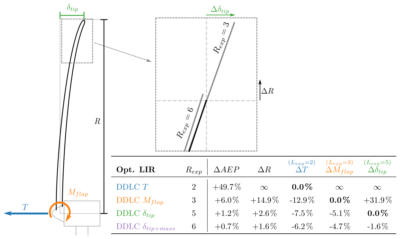
Figure 9Sketch of a turbine with the load/structural response outlined. The zoomed-in figure shows the radius increase (ΔR) and the change in tip deflection (Δδ_tip) for two different DDLCs (bold black line is the baseline). The table shows the relative change in power, radius and load/structural response for different DDLCs. R_exp=2 is a thrust constraint design, R_exp=3 is a flap moment constraint design, R_exp=5 is a tip-deflection constraint design and R_exp=6 is the tip deflection+constant mass constraint design.

Download

4.3 AEP-optimized rotor

As mentioned in Sect. 3, the variables considered for optimization of AEP are $C_{\mathrm{T}}\left(\stackrel{\mathrm{̃}}{V}\right)$ and $\stackrel{\mathrm{̃}}{R}$. In this formulation, C_T can be adjusted independently for each wind speed, which ideally can be achieved through blade pitch control. The relative radius $\stackrel{\mathrm{̃}}{R}$ couples the rotor operation across all wind speeds, as it is necessarily constant. Based on initial studies, the optimizer targets solutions with three distinct operational ranges, which, ordered by wind speed, are as follows:

• operation with maximum power coefficient (max C_P);

• operation at constraint limit (constant thrust T); and

• operation at the rated power.

This can be used to make C_T a function of $\stackrel{\mathrm{̃}}{R}$, thereby decreasing the optimization problem to an unconstrained optimization in one variable ($\stackrel{\mathrm{̃}}{R}$). The C_T function is given as

where the last equation needs to be solved to get C_T; the solution is a third-order polynomial, which is more easily solved numerically.

Figure 10Power and thrust curve for an AEP-optimized rotor (solid lines) where the DDLC exponent is R_exp=3, which is equivalent to a constraint on M_flap. The dashed line is the baseline rotor optimized for the max C_P below the rated power.

Download

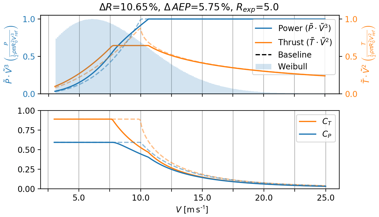
Figure 11Power and thrust curve for an AEP-optimized rotor (solid lines) where the DDLC exponent is R_exp=5, which is equivalent to a constraint on δ_tip. The dashed line is the baseline rotor optimized for the max C_P below the rated power.

Download

The only free parameter that needs to be determined to find the optimal AEP is $\stackrel{\mathrm{̃}}{R}$. The optimization problem can be reformulated as

The problem can be solved with most optimization solvers since the AEP can be computed explicitly if $\stackrel{\mathrm{̃}}{R}$ is given. The optimization problem was solved with the L-BFGS-B algorithm described in Zhu et al. (1997) though the use of SciPy (Millman and Aivazis, 2011).

Examples of the resultant power and thrust curves can be seen in Figs. 10 and 11, for DDLC(M_flap) and DDLC(δ_tip), respectively. Looking at Fig. 10 (R_exp=3) it is clear that the power and thrust curves have changed quite substantially, compared to the baseline Betz rotor (dashed curves). The thrust curve does not have a sharp peak anymore but rather a flat plateau. As mentioned in the Introduction this is often referred to as thrust clipping. It comes from the DDLC equation (Eq. 44) which shows that $C_{\mathrm{T}}\propto {\stackrel{\mathrm{̃}}{V}}^{-\mathrm{2}}$, and since thrust is proportional to $T\propto C_{\mathrm{T}}{\stackrel{\mathrm{̃}}{V}}^{\mathrm{2}}$, it means that the thrust is constant. As mentioned, the region where the rotor is thrust clipped is also where the DDLC is active, so opposed to the baseline and LIR rotor, the DDLC is active over a larger range of V. The larger range of V is also partly why ΔR=44.6 %, which is a huge increase. As a result, it also leads to a large increase, with ΔAEP=19.9 %. This is a very large change in $\stackrel{\mathrm{̃}}{R}$ and the feasibility of such a design is doubtful. As it is shown later, the change in maximum loads (see Fig. 13) leads to a significant change in loads with L_exp>R_exp.

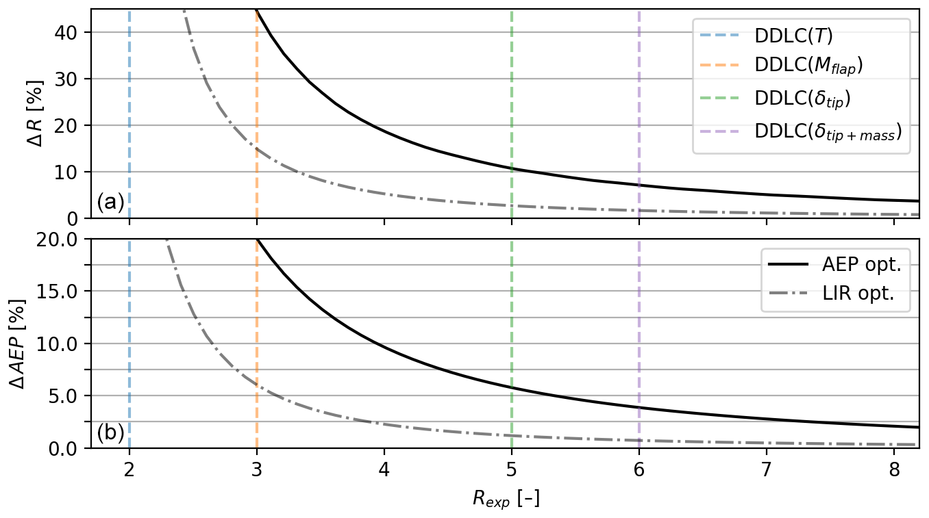
Figure 12DDLC exponent (R_exp) vs. (a) relative change in radius (ΔR) and (b) relative change in AEP ($\mathrm{\Delta }\stackrel{\mathrm{̃}}{\mathrm{AEP}}$). The plot contains both of the changes for the cases of the low-induction rotor (LIR opt.; dashed–dotted black line) and the AEP-optimized rotor (AEP opt.; black solid). The changes in both AEP and radius are much larger for the AEP-optimized rotor.

Download

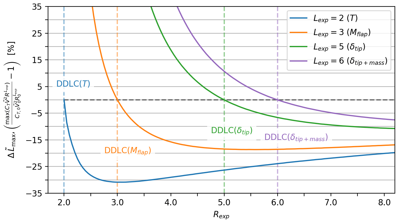
Figure 13DDLC R exponent (R_exp) vs. relative maximum load ($\mathrm{\Delta }{\stackrel{\mathrm{̃}}{L}}_{\max }$). The plot looks similar to Fig. 5 but $\mathrm{\Delta }{\stackrel{\mathrm{̃}}{L}}_{\max }$ is the change in maximum loading. As an example, when thrust (T) is −30.8 % for R_exp=3 it means that the maximum thrust (for any wind speed) is 30.8 % lower than the maximum thrust for the baseline (which happens just before the rated wind speed). Notice that the range for the y scale is much larger in this plot than for the power-capture-optimized rotor. The potential reduction is more, but it comes with the consequence that L_exp>R_exp grows faster even for high values of R_exp.

Download

A more realistic design for modern turbines is found in Fig. 11 (R_exp=5). Here the changes are fewer but still significant with ΔR=10.7 % and ΔAEP=5.8 %. It shows the same shape as the thrust-clipped curve, but now it is over a smaller range of V. As mentioned in the Introduction, thrust clipping was also found by Buck and Garvey (2015a) to be a beneficial way to lower CoE.

In Fig. 12 the relative change in R and AEP can be seen as a function of the DDLC R exponent. The plot both contains the result for the AEP-optimized rotor (AEP opt.; solid black line) and the low-induction rotor (LIR opt.; dashed–dotted gray line). The difference between the two is significant, especially for ΔAEP. The results for the AEP-optimized rotor are summarized in Fig. 14 with a table and a sketch that shows the relative changes. As was the case for power-capture optimization and LIR optimization, some values diverge when R_exp→2, and the results are found by investigating this limit. But since it has no practical value, further explanation is omitted here.

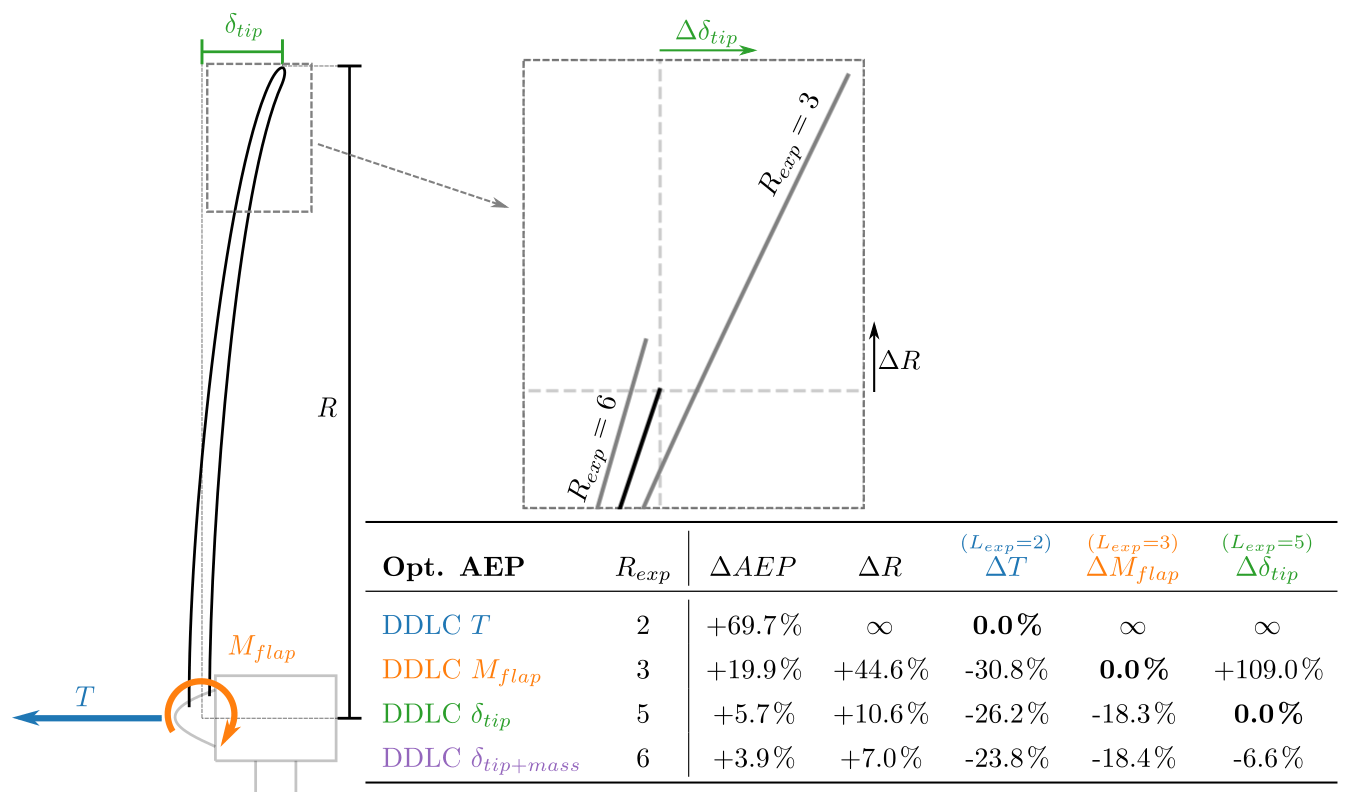
Figure 14Sketch of a turbine with the load/structural response outlined. The zoomed-in figure shows the radius increase (ΔR) and the change in tip deflection (Δδ_tip) for two different DDLCs (bold black line is the baseline). The table shows the relative change in power, radius and load/structural response for different DDLCs. R_exp=2 is a thrust constraint design, R_exp=3 is a flap moment constraint design, R_exp=5 is a tip deflection constraint design and R_exp=6 is tip deflection+constant mass constraint design.

Download

4.4 Summary of findings

In Table 1 the tables shown in Figs. 6, 9 and 14 are summarized. It compares the different optimizations to each other.

Table 1Overview of the optimization results from optimizing power capture (Opt. PC), low-induction rotor (Opt. LIR) and annual energy production (Opt. AEP).

Download Print Version | Download XLSX

As seen from the tables, the largest increase in ΔP∕AEP is found using AEP optimization, which also leads to the largest increase in rotor radius (ΔR). It also shows that using thrust clipping seems to be a better operational strategy than low induction, as the design-driving constraint can be met over a larger range of wind speeds and low induction is only needed around maximum thrust and not at low wind speeds.

In all three optimization cases, the optimization of the design with thrust constraint (DDLC(T); R_exp=2) leads to divergent values for ΔR and the loads. In all cases the result is found by investigating the behavior of the limit when R_exp→2. Since this is not thought to be of much practical value, the details are not provided here.

4.5 Limitation of the study and possible improvements

The study shows that for a rotor constraint by a static aerodynamic DDL there is a benefit to lowering the loading and increasing the rotor size in terms of power/AEP. But, as it was found by Bottasso et al. (2015), having a rotor with the same load constraint and increasing the radius does not mean that the cost is the same or that it is cost optimal. They found that the increase in AEP did not compensate for the added cost from increasing the rotor radius. This problem of cost vs. benefit is not directly addressed in this paper, but by the DDLC δ_tip+mass, a constraint in which the mass is kept constant. It is thought to be a better approximation for a rotor with a fixed price – but this assumption needs to be tested.

Another issue that is not taken into account in this study is the influence of the turbines self-weight. As was found by Sieros et al. (2012) the self-weight becomes more important for larger rotors. To accommodate for the added mass, a penalty could be added which should scale as $\stackrel{\mathrm{̃}}{R}$ or ${\stackrel{\mathrm{̃}}{R}}^{\mathrm{3}}$ for top head mass and static blade mass moment, respectively. As discussed above, there could also be a constraint implemented that will keep the mass or the mass moment in the optimization. Again this is a limitation of the study.

The fidelity of the models is also a limitation. Even though 1-D aerodynamic momentum theory is a common approximation to do for first-order studies in rotor design, it is well known that the constantly loaded rotor is not possible to realize, and when losses are included the constantly loaded rotor is not the optimal solution anymore. At the same time, if it was possible to decrease the load at the tip more than at the root, it would lead to less tip deflection than a constantly loaded rotor with a similar C_T. Extending the model to be able to handle radial load distribution is one way of adding detail to the model that could lead to even larger improvements. It could be done through the use of blade element momentum (BEM) theory.

For modern turbine design, it is often the case that the structural design is determined by the aeroelastic extreme loads, such as extreme turbulence or gusts. With the simplicity of the models in this study, this is not taken into consideration. But if the extreme load happens in normal operation there will likely be a direct relationship between the steady and extreme loads, meaning that a decrease in steady loads will also lead to a decrease in the extreme load. This is an assumption that should be tested in future work. If the design-driving load is happening in nonoperational conditions, e.g., extreme wind in parked conditions, grid loss or subcomponent failure, then the analysis tool cannot be directly applied.