3.1 Area of interest and time period

The offshore part of NEWA covers the European Union, associated states, and Turkey from the coastline and at least 100 km offshore. For the WRF model, the simulations are performed for 10 separate subdomains and later merged to provide one unified atlas (Fig. 1). The WRF modelling covers 30 years from 1989 to 2018. For the satellite data collection, processing and analysis, it is convenient to select an area of interest within latitudes (here 33.5 to 72.2^∘ N) and longitudes (here 19.4^∘ W to 47^∘ E).

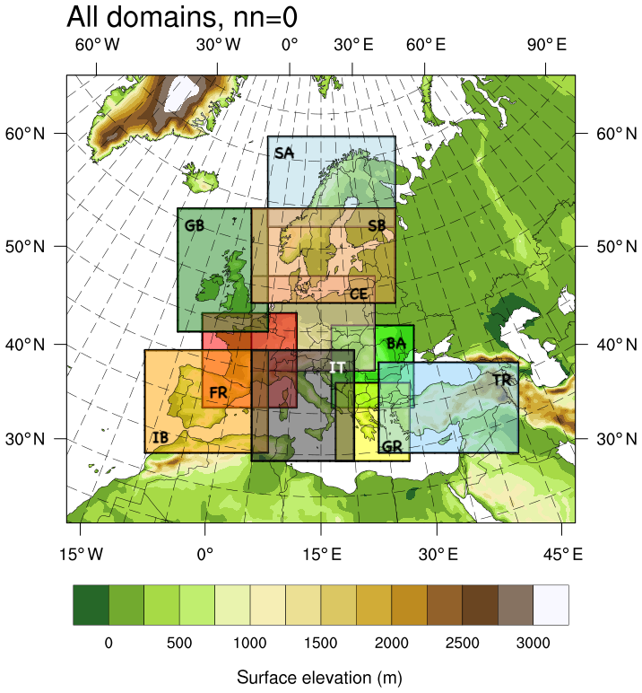
Figure 1The WRF modelling domain with 10 subdomains used in the production of the New European Wind Atlas.

3.2 ASCAT and SAR ocean wind processing

The scatterometer ASCAT is on board the meteorological MetOp-A and MetOp-B satellites observing from 2007 and 2012, respectively, to present. MetOp-C was launched in 2018 although its data are not used in the present study. All are operated by the European Organisation for the Exploitation of Meteorological Satellites (EUMETSAT). The Level 3 data obtained through the Copernicus Marine Environmental Monitoring Service are the coastal stress equivalent wind product (WIND_GLO_WIND_L3_NRT_OBSERVATIONS_012 _002). They include wind speed and wind direction at 10 m height above sea level at a spatial resolution of 12.5 km (De Kloe et al., 2017; CMEMS, 2019). Depending on the area of interest, satellite overpass times can range from two to four per day, while the measurements are considered instantaneous (CMEMS-OSI-PUM-012-002, 2019). Near coastlines, quality control omits pixels contaminated by land that cause fundamentally different scattering than ocean waves. Level 1 Wide Swath Mode (WSM) acquisitions from the Envisat ASAR (Advanced SAR) mission, from 2002 to 2012, are collected in their entirety for the area of interest. The scenes used in this study include co-polarized VV and HH scenes (VV is vertical receiving and vertical transmitting, and HH is horizontal receiving and transmitting). Envisat was a research mission of the European Space Agency (ESA).

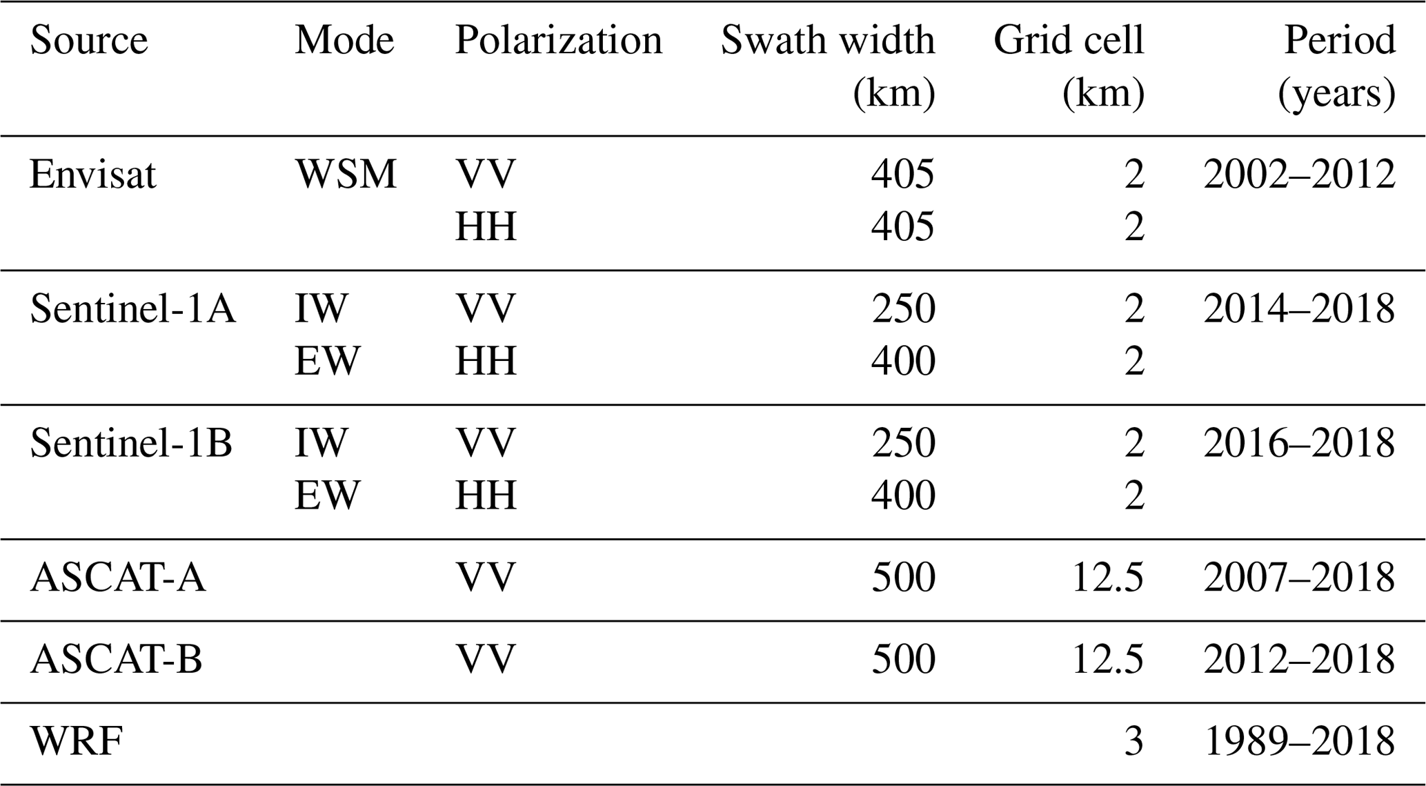
Level 1 Extra Wide (EW) and Interferometric Wide (IW) mode acquisitions from the Sentinel-1A mission (2014–present) and Sentinel-1B (2016–present) are collected in their entirety for the area of interest. The scenes used in this study include EW and IW mode and VV and HH polarization. Sentinel-1A/B are parts of Copernicus, the European Commission's monitoring programme. Table 1 lists the source data from ASCAT, Envisat and Sentinel-1.

Table 1List of source data for the European seas between 1989 and 2018 for ASCAT, SAR and WRF.

Download Print Version | Download XLSX

ASCAT, Envisat and Sentinel-1 are polar-orbiting satellites. The number of samples of ocean wind data in any pixel (grid cell) depends upon the data recordings in time and space. For Envisat this was inhomogeneous due to various research priorities in the beginning of the mission. During later years (2008 to 2012), recording was high and consistent in the area of interest. ASCAT-A/B and Sentinel-1A/B are operational monitoring satellites and have frequent coverage in the entire domain since launch. For all satellites, there are more samples available at higher latitudes due to the polar-orbital paths. The SAR wind retrieval is based upon calibrated radar backscatter values (the normalized radar cross section) and application of the GMF CMOD5.N (Hersbach, 2010). CMOD5.N gives the equivalent neutral wind at 10 m height above sea level. This is for radar data in VV polarization. There is no GMF for HH data; therefore a conversion, the so-called polarization ratio linking the VV and HH data together, needs to be applied before wind retrieval. For HH data, the polarization ratio of Mouche et al. (2005) is selected. The a priori wind directions needed to perform wind retrieval are selected at 10 m height from the NCEP/NCAR Climate Forecast System Reanalysis (CFSR) reanalysis data until 2010, and the Global Forecast System (GFS) data are used from 2011 onward. To match the SAR images, an interpolation of wind directions is performed. The SAR Ocean Products System (SAROPS) software from Johns Hopkins University Applied Physics Laboratory and National Ocean and Atmosphere Agency (JHU APL and NOAA) is used for the processing (Monaldo et al., 2014), which occurs operationally at DTU Wind Energy; all wind retrievals are openly available through https://satwinds.windenergy.dtu.dk/ (last access: 24 March 2020). In regions with sea ice, ocean winds cannot be retrieved, and thus these areas are masked out using the National Ice Center's Interactive Multisensor Snow and Ice Mapping System (IMS) with daily data at 4 km resolution (National Ice Center, 2008).

Satellite winds retrieved at 10 m height are averaged into wind resource statistics using the software for SAR-based wind resource assessment (Hasager et al., 2008, 2011; Ahsbahs et al., 2019) and for ASCAT using the methodology presented in Karagali et al. (2018b). Wind turbines offshore have hub heights at around 100 m height. Therefore, an extrapolation of wind speed from 10 to 100 m height is applied. Previous investigations show that applying a long-term stability correction is superior to a neutral logarithmic wind profile in the Baltic Sea (Badger et al., 2016) and in the North Sea (Karagali et al., 2018a). For the NEWA offshore wind atlas, the extrapolation is performed similarly to Karagali et al. (2018a, b) using 10 years of WRF model simulations from Nuño Martinez et al. (2018) for the long-term stability correction.

3.3 Mesoscale modelling

The WRF model (Skamarock et al., 2008) used for the production run of the New European Wind Atlas is a limited-area weather forecast model. The WRF model is a public domain, open-source modelling system, which has previously been used to produce a wind atlas for South Africa (Hahmann et al., 2015b), the North Sea and Baltic Sea (Hahmann et al., 2015b), and Denmark (Peña and Hahmann, 2017) and wind statistics for Europe (Nuño Martines et al., 2018).

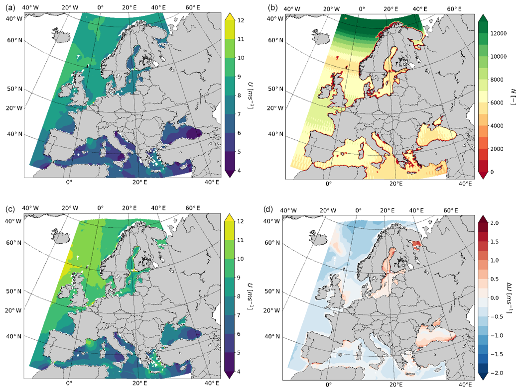
Figure 2For ASCAT the mean wind speed (m s⁻¹) at 10 m height (a), number of samples (b), mean wind speed at 100 m including long-term stability correction for extrapolation (c) and difference in wind speed at 100 m a.m.s.l. height based on long-term stability correction minus neutral wind profile assumption (d) are shown.

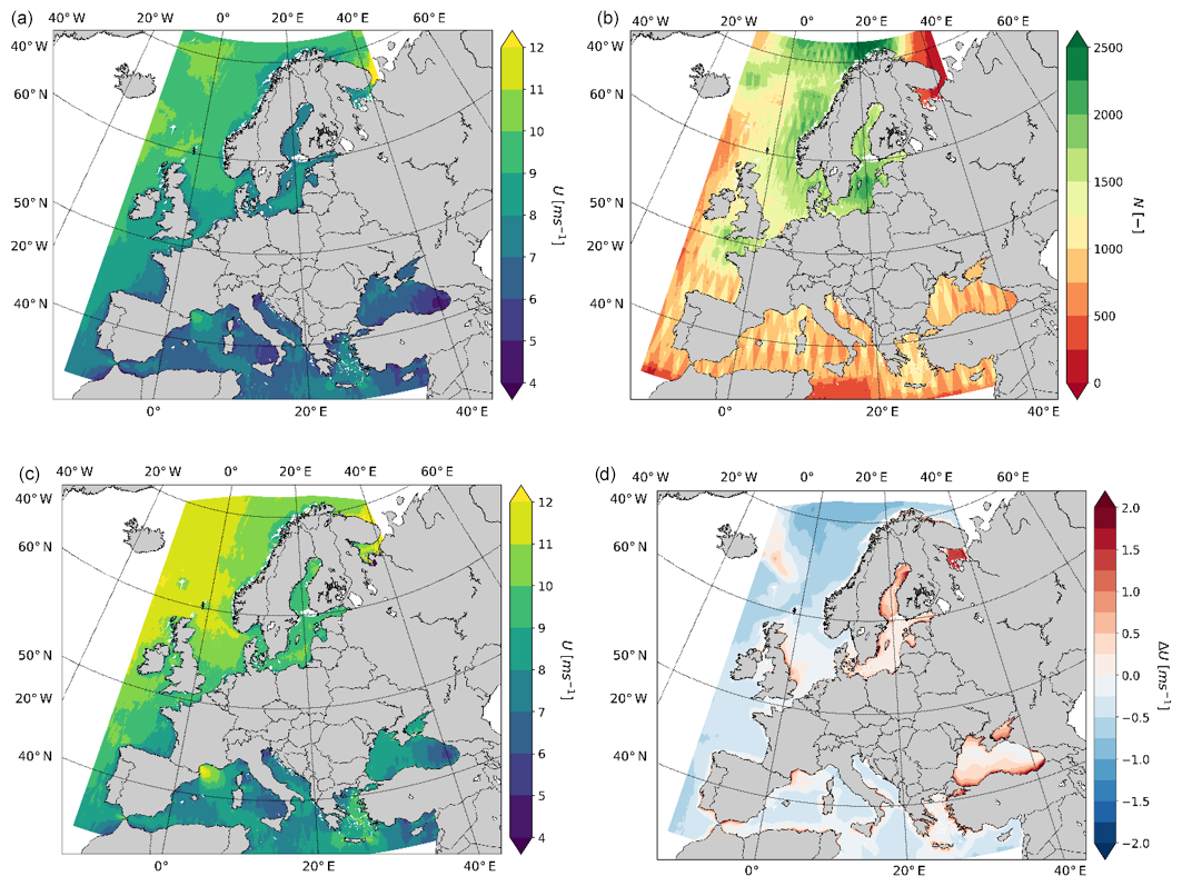
Figure 3For Envisat ASAR and Sentinel-1 combined mean wind speed (m s⁻¹) at 10 m height (a), number of samples (b), mean wind speed at 100 m a.m.s.l. including long-term stability correction for extrapolation (c) and difference on wind speed at 100 m a.m.s.l. height based on long-term stability correction minus neutral wind profile assumption (d) are shown.

The production run for NEWA (see Fig. 1) was computed on the HPC cluster MareNostrum at the Barcelona Supercomputing Center and on HPC Cluster EDDY at the University of Oldenburg. In order to determine the optimal model scheme and forcing, surface input, and land surface model, a series of sensitivity tests were conducted and compared to tall meteorological mast data masts and lidar data in northern Europe and the North Sea. No setting was optimal for all, so a compromise was made, which provided the best verification statistics (see Witha et al., 2019, for more details). In brief, the production run was set up for 10 separate WRF domains, which shared the same outer domain and map projection, and later merged to provide one unified atlas (https://map.neweuropeanwindatlas.eu, last access: 24 March 2020). The WRF model used was a modified version of 3.8.1, set up with the Mellor–Yamada–Nakanishi–Niino (MYNN) planetary boundary layer (Nakanishi and Niino, 2009) and Monin–Obukhov surface layer (Monin and Obukhov, 1954) schemes. Forcing for the simulations was from ERA5 reanalysis (ERA5, 2017) at $\mathrm{0.3}{}^{\circ }\times \mathrm{0.3}{}^{\circ }$ grid spacing and OSTIA sea surface temperature (Donlon et al., 2012) at 1∕20^∘ grid spacing. The CORINE land cover data at 100 m resolution were used to define the land use classes (Copernicus Land Monitoring Service, 2019), except for areas they do not cover, in which case ESA CCI data are used. The NOAH land surface model and icing WSM5 plus ice code and sum of cloud and ice humidity are used. The WRF simulations used three nested domains at 27, 9 and 3 km and 61 vertical layers, with 8 d overlapping runs using spectral nudging with 24 h spin-up (see Hahmann et al., 2020, for details on the technique). There are 20 model levels below 1 km, and the lowest levels are located at 5.6, 21.8, 40.4, 56.6, 72.8, 90.7, 113.2, 140.1, 170.7, 205.3 and 244.5 m above ground level. The years covered and spatial resolution are listed in Table 1.

4.1 Satellite-based offshore wind speed maps

Figure 2 shows the offshore wind speed maps for the European seas based on the entire archive of ASCAT at 10 and 100 m height, the number of samples, and wind speed difference at 100 m using extrapolation with long-term stability correction minus neutral profile extrapolation. Similar results for SAR are shown in Fig. 3.

The same colour scale is used for ASCAT and SAR in Figs. 2 and 3, except for the number of samples due to the difference in sample maxima between ASCAT and SAR. The polar orbits result in more frequent sampling at higher latitudes. The harlequin pattern in sampling is due to the ascending and descending orbits for both ASCAT and SAR, but it is most noticeable for SAR due to the swaths and orbital settings.

For the European seas, the number of samples in the grid cells for ASCAT is greater than 4000 and in most places greater than 6000, up to more than 12 000 at high latitudes (see Fig. 2). The number of samples for SAR is between 500 and 2500 (see Fig. 3). For the WRF model, the number is constant at all locations covered with 525 912 samples (every 30 min from 1989 to 2018).

The mean wind speed consistently shows higher values for the 100 m height than 10 m height in both ASCAT and SAR. The wind speed difference maps at 100 m based on long-term stability correction minus neutral wind profile assumption show very similar spatial patterns between ASCAT and SAR, as expected. The variation is up to ±2 m s⁻¹ with high positive values in the Baltic Sea and Black Sea and with high negative values in the Norwegian Sea. Positive values occur for stable conditions. The continental climate dominating the flow in the Baltic Sea and the Black Sea causes the variations. Negative values occur for unstable conditions prevalent in the Norwegian Sea and in the Mediterranean Sea. According to Kara et al. (2009) the overall stability in the Mediterranean Sea is slightly unstable. In the North Sea, a gradient is observed with slightly negative values along the continental coast and positive values along the UK coast. This corresponds well with the average stability over the North Sea (Peña and Hahmann, 2012), where unstable conditions prevail along the continental coast and stable conditions prevail near the UK. The Mediterranean Sea has mixed wind speed difference variations dominated by moderately negative values in the central part and positive values in the Greek archipelago and the French Riviera.

4.2 WRF offshore wind speed map

The long-term offshore wind speed map at 100 m height in the European seas based on the WRF production run is shown in Fig. 4, using the same colour scale as for ASCAT and SAR in Figs. 2 and 3.

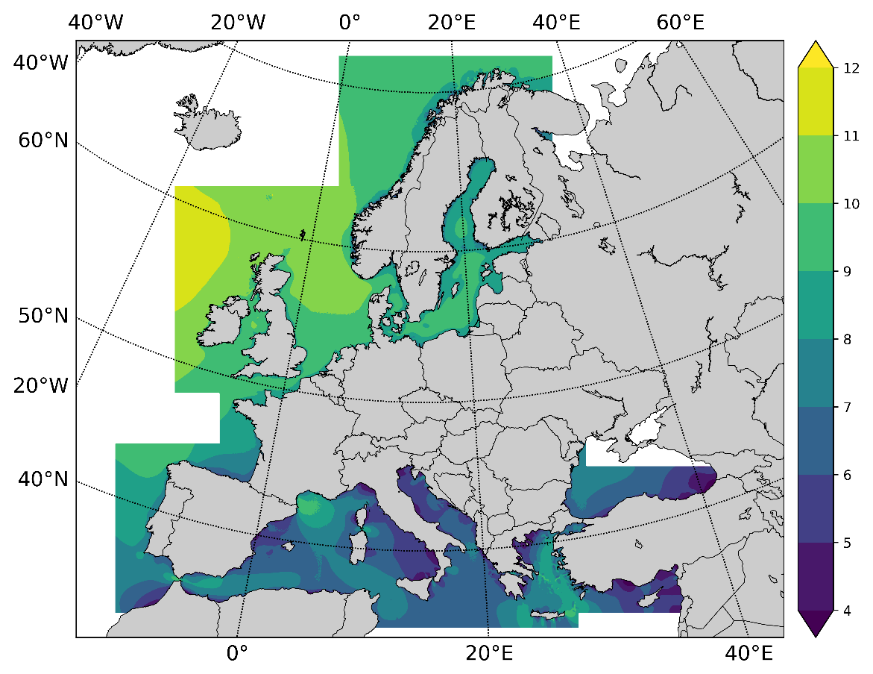
Figure 4WRF New European Wind Atlas production run mean wind speed (m s⁻¹) at 100 m height for 1989 to 2018 with 3 km spatial grid spacing.

ASCAT and WRF have many similarities in the spatial wind speed patterns and the range of mean wind speeds at 100 m height. The SAR mean wind speed at 100 m height appears to be higher than ASCAT and WRF. Furthermore, SAR shows more fine-scale spatial variations than both ASCAT and WRF.

4.3 Comparison of offshore mean wind speed maps at 100 m height

Comparisons of the ASCAT, SAR and WRF mean wind speed maps at 100 m height performed using the long-term stability-corrected versions from ASCAT and SAR are shown in Fig. 5. ASCAT versus WRF (panel a) shows lower differences in mean wind speed than SAR versus WRF (panel b). ASCAT minus SAR (panels c) shows a consistent negative bias of winds from SAR, except for some artefact in ASCAT near the Dutch coastline, attributed to higher backscatter from the surface due to the congestion of large ships to and from Rotterdam (notice distinct yellow area in Fig. 2 that without ships would be green; in other words, the high backscatter translates into falsely high wind speed).

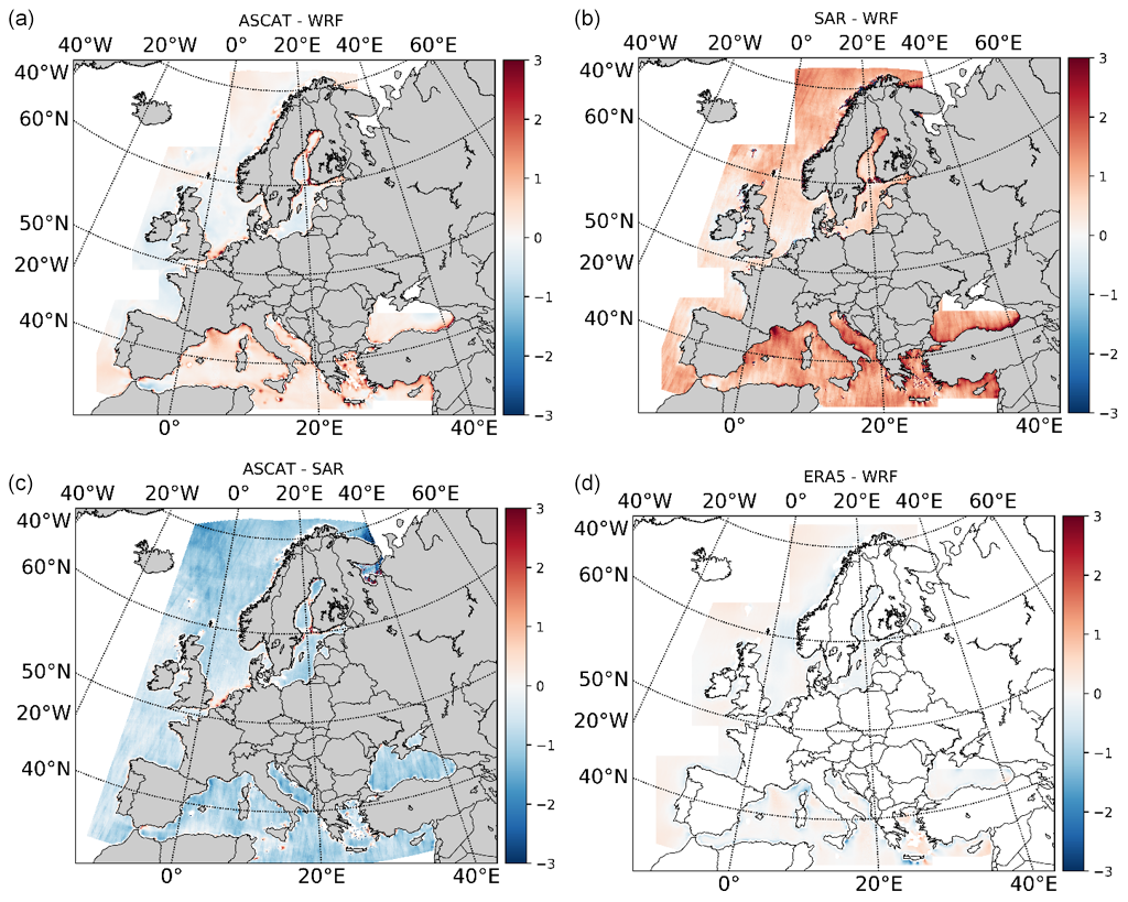
Figure 5Comparison of mean wind speed (m s⁻¹) at 100 m height: ASCAT minus WRF (a), SAR minus WRF (b), ASCAT minus SAR (c), and ERA5 minus WRF (d).

The ERA5 mean wind speed at 100 m height is included for comparison with WRF in Fig. 5 (panel d). Only grid cells with more than 95 % sea according to the ERA5 land mask are included. The mean wind speed difference map of ERA5 minus WRF shows some variations. There are both large positive and large negative values in the Mediterranean Sea. The differences are smaller in the northern European seas. Along several coastlines such as the Norwegian Sea, the Atlantic Sea and the Mediterranean Sea large differences are found between the two datasets. These are attributed to the lack of ability in ERA5 to properly resolve the coastal atmospheric flow phenomena such as land–sea breeze and flow intensification. See Beal et al. (2015) for further details on coastal atmospheric flow phenomena observed in SAR. ERA5 has a coarse spatial resolution omitting islands such as Bornholm and the Isle of Man. Coastal atmospheric flow phenomena near Crete are investigated in Sect. 5.

Please note the number of samples and the grid spacing are different. WRF has 30 min values from 30 years (525 912 samples) with 3 km resolution. ERA5 has hourly values from 30 years (262 956 samples) with about 27 km resolution.

With regards to spatial resolution, it is obvious that SAR resolves finer spatial detail than other products. From spectral analysis of SAR vs. scatterometer winds, it was found that SAR resolves around 4 km features, and the scatterometer resolves around 25 km features (Karagali et al., 2013b). The latter is comparable in scale to what the WRF model at 3 km grid spacing resolves, i.e. around 20 km (Skamarock, 2004). ERA5 resolves scales around 150 km. The use of structure functions and spectra from other numerical weather models has shown the effective model resolution to be about 6 times lower than the size of the grid cell (Frehlich and Sharman, 2008).

The wind speed difference error distributions between wind speed at 100 m height for ASCAT minus WRF, SAR minus WRF, ASCAT minus SAR and ERA5 minus WRF are shown in Fig. 6. ASCAT minus WRF has a slightly positive bias and narrow range. ASCAT minus SAR has a negative bias and moderate range. SAR minus WRF has a positive bias and broad range. The narrow range is expected for products that resolve similar length scales while broader ranges are expected for products that resolve different length scales. The results shown in Fig. 6 support this very well, as ASCAT and WRF resolve similar scales and SAR and WRF resolve very different scales. SAR generally shows higher wind speeds than ASCAT and WRF. The long positive tails of ASCAT minus WRF and SAR minus WRF are explained by coastal winds in the Mediterranean Sea. ERA5 minus WRF has a slightly positive bias and narrow range. All probability density distributions except ASCAT minus SAR show bimodal distributions explained by the differences in area of the northern seas and Mediterranean Sea; see Fig. 5.

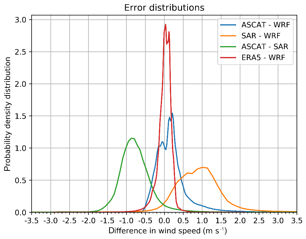
Figure 6Error distribution of the wind speed difference at 100 m a.m.s.l. for ASCAT minus WRF, SAR minus WRF, ASCAT minus SAR and ERA5-WRF. The distributions are normalized so the area below the curves sums to 1.

Download

5.1 Motivation and aim

The motivation for presenting a case study is twofold. Firstly, by looking into a small area of interest, spatial details in winds observed can be analysed and used as an example for characterizing the SAR and WRF data sources. More specifically, the goal of this case study is to study the interaction between large-scale flow and orography. The second motivation is to stimulate interest for further investigation using the different data sources at other locations in Europe and outline the methodology.

5.2 Selection of data

The sea surrounding western Crete is chosen due to interesting mesoscale flow patterns. Figures 7, 8, 10 and 11 show spatial wind patterns in the area. The area of investigation is located between 23.4 to 24.8^∘ E and 34.6 to 36.0^∘ N. The SAR scenes available from the database satwinds.dtu.dk at DTU Wind Energy are selected. To have spatial consistency between SAR and WRF, only SAR scenes that fully cover the area (consecutive scenes are merged) are selected.

Figure 7Mean wind speed (m s⁻¹; 2002–2018) at 10 m a.m.s.l. for (a) WRF and (b) SAR. All 549 coinciding scenes are used in both datasets.

There are 549 SAR scenes between 2002 and 2018 in total from Envisat and Sentinel-1. Only coinciding WRF data are selected. The SAR and WRF mean wind speeds at 10 m height are displayed in Fig. 7. Some wind features are similar in SAR and WRF, e.g. lower wind speeds south and north of Crete close to the shore. A distinct jet south of the island is much more pronounced in the WRF data than in SAR. Figure 7a shows the height contour lines from the elevation map used in the WRF model. To characterize the complex landscape in Crete, a more detailed elevation map is embedded in the SAR map in Fig. 7b. Small-scale elevation features not represented in the WRF model may explain wind speed differences between WRF and SAR. The jet could be weaker or absent since the fine-scale elevation features, neglected in WRF, block the atmospheric flow. For instance, what is a simple valley without any obstacles in WRF orography, in reality (and therefore in SAR data), could be blocked by a small mountain range. Koletsis et al. (2009) demonstrated the sensitivity of gap wind speeds in a mesoscale model to the changes in the elevation.

The variability in coastal flow around Crete depends highly on the wind direction. Two of the prevalent wind directions are of particular interest – namely northerly and westerly winds. Northerly winds over Crete are associated with the so-called Etesian wind often present in the region during summer and known to produce gap flows between the two large mountains in the east side of the island (Lefka Ori) and in the centre (Idi) (Koletsis et al., 2010). Westerly winds in this region have been associated with trapped lee waves (Miglietta et al., 2013).

As already stated, the goal of this case study is to demonstrate the interaction between large-scale flow and orography. It is necessary to choose situations where the upwind flow conditions are simple. This is to avoid wind conditions such as low wind speed with poorly defined direction, anti-cyclonic situations and local flows, e.g. sea breezes that could create a complicated wind field that would be difficult to interpret. Therefore, the wind speeds should be sufficiently high, and the wind direction should be representative for the entire domain.

To determine a representative flow direction, ERA5 wind speeds and directions extracted at the locations indicated in Fig. 8 are used. Figure 8 also shows the mean wind speed from the 549 coinciding ERA5 model simulations. ERA5 resolves the mean wind speed with much less spatial detail than WRF (compare Figs. 8 and 7b). The average wind speed at three points (A, C, E) is required to be above 3 m s⁻¹. For the wind direction, the centre location upstream (B for northerly, D for westerly) should be within 30^∘ of that direction. We further require that the neighbouring upstream points do not differ by more than 20^∘ from the centre. Figure 9 illustrates the flow chart used for classification.

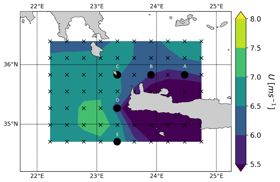
Figure 8Mean wind speed (m s−1) from ERA5 for 549 cases collocated with SAR scenes around Crete with points used for extracting wind speed and direction for classification. The five locations A to E are mentioned in the text.

The mean wind speed maps based on SAR and WRF for 59 cases of northerly and 57 cases of westerly flows are presented in Fig. 10. For northerly flow, notable differences exist between the SAR and WRF maps. The WRF winds show strong shadowing at 24^∘ E and a pronounced jet-like structure at 24.5^∘ E. These features are present in SAR as well, but much less pronounced. For westerly flow, good agreement between SAR and WRF is noted. Areas of increased wind speed to the south and the north are visible in both maps. A stagnation point area of low wind speed is located on the western side of Crete in both SAR and WRF maps. Stronger winds may increase surface water mixing, causing colder sea surface temperature (not shown).

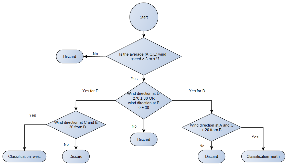
Figure 9Flow chart for selection of cases classified as winds from northern and western directions.

Download

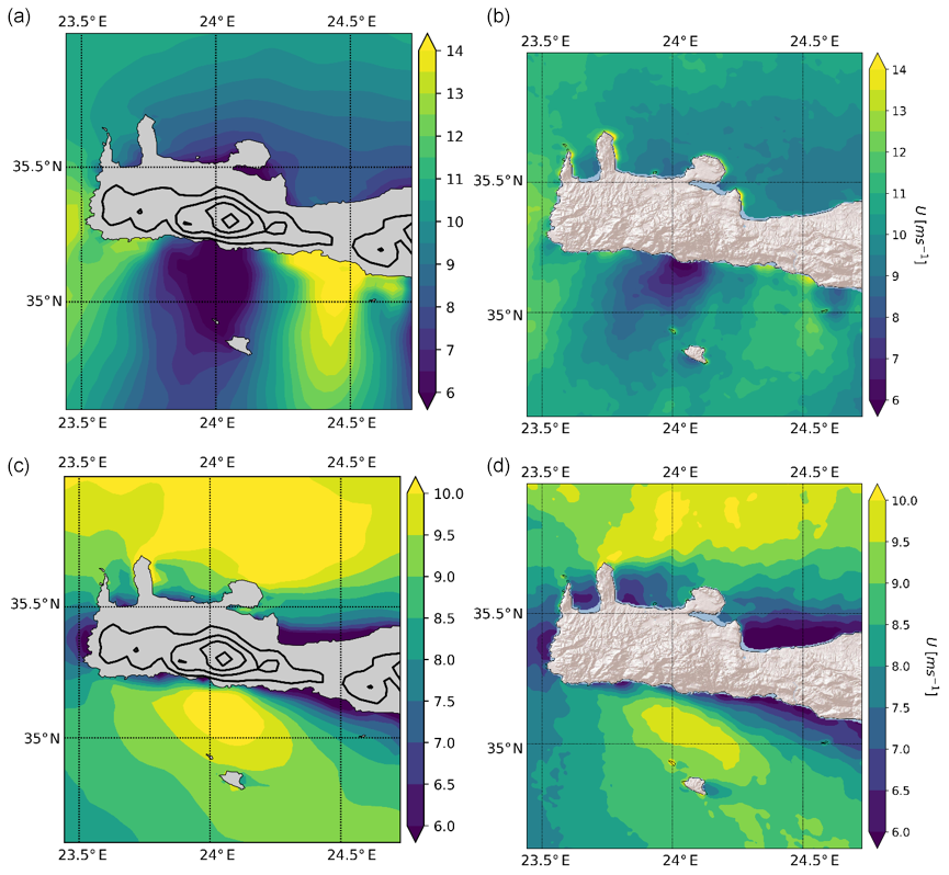
Figure 10Mean wind speeds (m s⁻¹) from WRF (a, c) and SAR (b, d) at 10 m. (a, b) Northerly flow based on 59 collocated cases from 2002 to 2018. (c, d) Westerly flow based on 57 collocated cases from 2002 to 2018.

To clarify further similarities and discrepancies between SAR and WRF, two individual examples are chosen and compared to WRF (see Fig. 11): one case of northerly flow from 5 July 2017 at 04:24 UTC and one case of westerly flow from 6 May 2017 at 04:24 UTC.

The northerly flow SAR case (Fig. 11b) contains significant atmospheric waves. Although some evidence for atmospheric wave activity is also identified in the WRF data, namely periodic changes of flow over time (not pictured), no wave structure similar in wavelength to the one visible in SAR is identified in WRF. This could be because topography of the appropriate resolution is not present in the WRF model and thus cannot be resolved in the mode solution. In addition, the WRF model grid is too coarse to resolve the scale of the observed waves. The wind speed maxima in SAR and WRF compare well, as do the minima for the northerly flow case (Fig. 11a, b). The much weaker jet identified in the average of northerly flows in SAR vs. WRF (in Fig. 11a, b) can, in part, be explained by the gravity wave amplitude maxima not occurring at the same location. The averaging of out-of-phase waves can lead to destructive interference and result in the average sum of lower values in SAR. In contrast, WRF appears to simulate only the maxima of the unresolved waves.

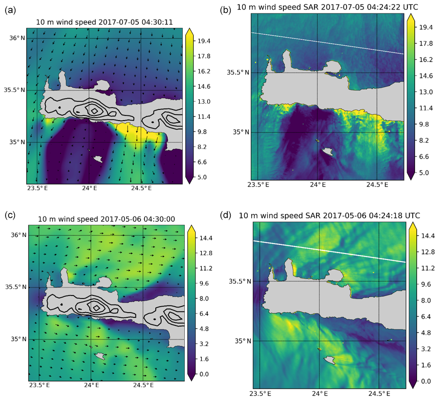
Figure 11Wind speed (m s⁻¹) from WRF data (a, c) and SAR data (b, d). (a, b) Northerly flow on 5 July 2017, 04:24 UTC. (c, d) Westerly flow on 6 May 2017, 04:24 UTC (the white lines in SAR panels are consecutive scene borders).

The westerly flow case for SAR and WRF (Fig. 11c, d) also shows atmospheric wave activity. However, in this case the waves seem to have a longer wavelength and therefore could – although imperfectly – be reproduced in WRF; WRF still shows significantly longer wavelengths than SAR.

In summary, the orography in WRF is somewhat simplified and therefore significant features playing critical role in complicated flows are omitted. Another direction of investigation is to assess whether the atmospheric stability in the flow before it arrives at the obstacle has the correct representation in WRF. Meteorological observations are unfortunately not available for comparison.

The atmospheric stability from WRF has been investigated. We use the stability classes derived from the Obukhov length following Gryning et al. (2007) and map the stability at the time of the two cases shown in Fig. 11. The results are presented in Fig. 12. For the case with winds from the north, the inflow is very unstable at the northern shore of Crete, but in the high-speed jet south of Crete the flow is neutral. In the low-speed zone south of Crete there is a complicated pattern of atmospheric stability – with a large zone of very unstable flow. For the case with winds from the west, the inflow (west of Crete) is again very unstable, and the wind speed maxima are again associated with neutral stability conditions, but this time in the low-wind-speed zones near the coastline north and south of Crete very stable stratification is found.

Figure 12Stability class following Gryning et al. (2007) in WRF for the cases with winds from the north (a) and from the west (b).

The results in Fig. 12 show a snapshot of stability in time; however, the focus on this paper is the climatological properties. Therefore, the next question arises – are these stability patterns typical? To answer this question, we analyse the stability patterns in the WRF dataset that coincides with SAR scenes (Fig. 10). The stability distribution for the 59 cases of northern winds (not shown) is characterized by a high probability of very unstable flow both in the inflow (north of Crete) and in the low-speed zone. A small increase in the frequency of neutral winds in the jet zone is also noted. This result allows us to argue that the conclusions from Fig. 12 can be generalized. The average stability for the 57 cases of westerly winds (not shown) has very unstable inflow to the west of Crete as in Fig. 12. The high-wind areas are associated with neutral or near-neutral stratification while the low-wind zones along the coastlines to the north and south have very unstable stratification. This leads us to conclude that the pattern in stability for westerly flow is similar between the single case (Fig. 11) and average (Fig. 10) except very close to the coastline for low wind speeds.