2.1 Wake model

The impact of wakes on turbine power production is modeled using the FLORIS engineering wake modeling tool (NREL, 2019c). Specifically, the Gaussian wake model developed by Bastankhah and Porté-Agel (2014, 2016) and Niayifar and Porté-Agel (2016) is used to model the velocity deficits and wake profile. This model includes the ambient turbulence intensity (TI) as a parameter that helps determine the rate of wake recovery and the wake expansion. Wake deflection caused by yaw misalignment is modeled using the wake deflection model of Bastankhah and Porté-Agel (2016), based on the Reynolds-averaged Navier–Stokes equations. More information about the wake and wake deflection models available in FLORIS can be found in Annoni et al. (2018) or at https://floris.readthedocs.io (last access: 1 April 2020).

An example of the wakes produced by a two-turbine array with five rotor diameter (D) spacing using the abovementioned wake model, with mean free-stream wind speed U=8 m s⁻¹ and a TI value of 10 %, is provided in Fig. 1. The wake behavior is shown for the baseline case of zero yaw misalignment as well as with a positive 20^∘ yaw offset applied to the upstream turbine. Note that a positive yaw offset corresponds to a counterclockwise rotation of the turbine relative to the wind direction.

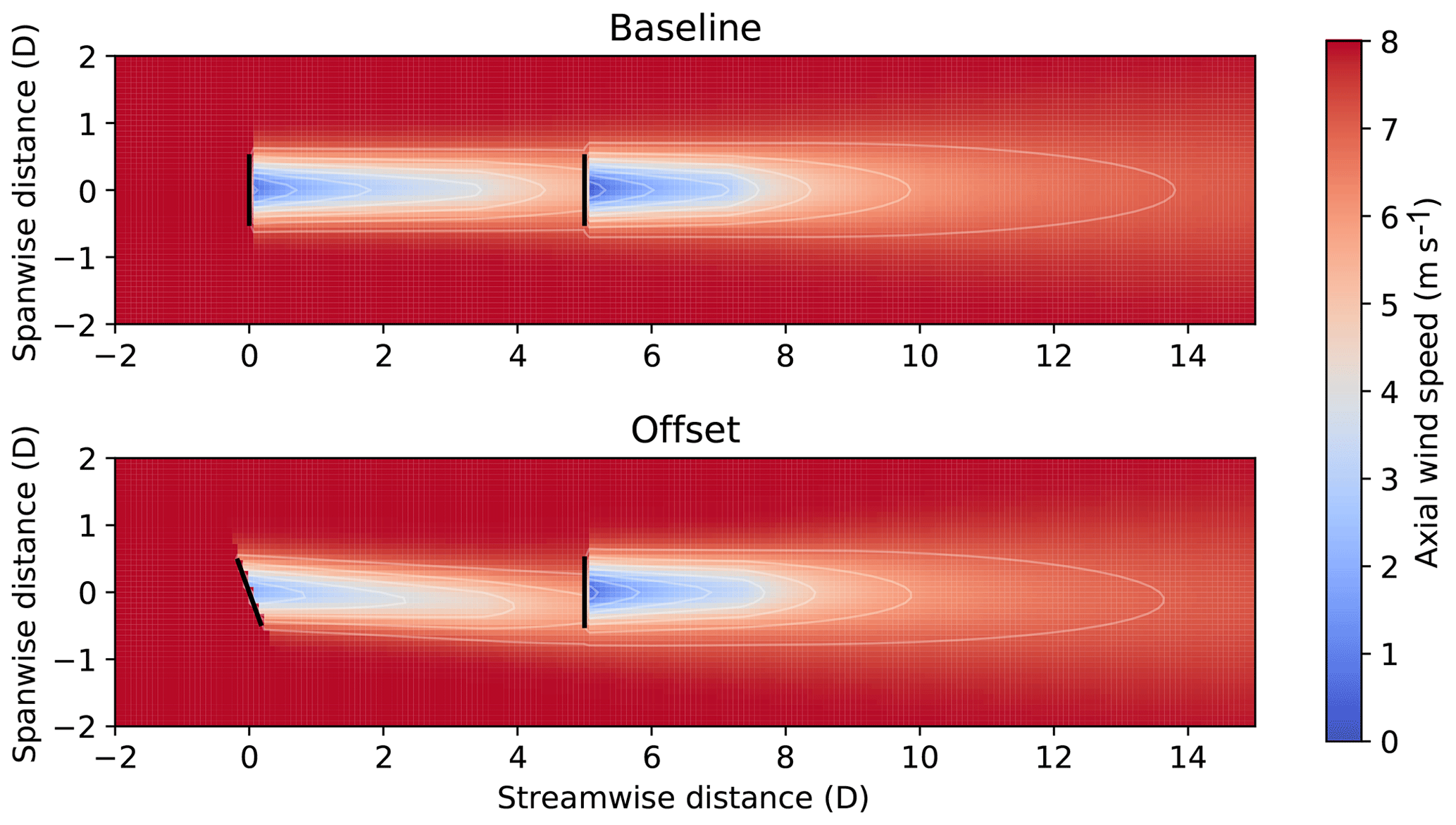
Figure 1Examples of wakes for a two-turbine scenario with five rotor diameter (D) spacing using FLORIS. In the baseline case, both turbines are aligned with the wind direction. For the offset case, the upstream turbine has a yaw offset of 20^∘.

Download

2.2 Wind turbine

The wake behavior and power production computed by FLORIS rely on a simplified wind turbine model, which is based on the NREL 5 MW reference wind turbine model in this research (Jonkman et al., 2009). The NREL 5 MW reference turbine has a rotor diameter of 126 m and a hub height of 90 m. All analysis in this paper is based on simulations with a mean free-stream wind speed of U=8 m s⁻¹, corresponding to a power production of 1.81 MW (rated wind speed for the NREL 5 MW reference model is 11.4 m s⁻¹). With U=8 m s⁻¹, the NREL 5 MW reference turbine operates in region 2, where power production is maximized and thrust is relatively high (the coefficient of thrust C_T=0.762), conditions in which wake losses are high and wake steering is most effective.

To model the impact of yaw misalignment on power production, a simple cosine power-law relationship is used in conjunction with the standard power equation in FLORIS:

where γ is the yaw offset and the exponent p describes how quickly power decreases with increasing yaw misalignment. A value of p=1.88 is used here, based on fitting Eq. (1) to data from a LES, as reported by Gebraad et al. (2016).

2.3 Yaw controller

Yaw control is simulated using simple logic based on the yaw controller model described by Bossanyi (2018). A slowly varying wind direction signal is formed by low-pass filtering the measured wind direction, given by the sum of the wind vane signal and the nacelle position, using a first-order filter with a time constant of 35 s. When the magnitude of the difference between the filtered wind direction and the nacelle position exceeds a threshold of 8^∘, the turbine begins yawing toward the direction of the filtered wind direction at the yaw rate of 0.3^∘ s⁻¹ defined for the NREL 5 MW reference turbine (Jonkman et al., 2009). Once the difference between the current yaw position and the slowly varying filtered wind direction reaches zero or changes sign, the turbine stops yawing until the error threshold is exceeded again. The values of the error threshold and yaw rate parameters used here are equivalent to those presented by Bossanyi (2018). However, instead of the 30 s filter time constant described by Bossanyi (2018), a slightly longer time constant of 35 s is used here, which results in yaw activity similar to that of a commercial wind turbine used in the wake steering experiment discussed by Fleming et al. (2019).

2.4 Yaw offset controller

For a specific wind direction, optimal yaw offsets are found for the upstream turbine in a turbine pair by determining the offset that maximizes the sum of the power produced by the two turbines using FLORIS. Because of the practical challenges of switching between large positive and negative yaw offsets for small changes in wind direction as well as the relative benefits of positive yaw misalignments, only positive offsets are considered here. For example, Damiani et al. (2018) show that blade root bending moment fatigue is reduced with positive yaw misalignments but increases with negative yaw misalignments. Additionally, LES shows that positive yaw misalignments are more effective at increasing power production as a result of the behavior of large-scale trailing vortices that help steer the wake, as explained by Fleming et al. (2018), as well as the impact of the Coriolis force on wake deflection, discussed by Archer and Vasel-Be-Hagh (2019). To further reduce the impact of wake steering on turbine loads, we limit yaw offsets to 20^∘ (Damiani et al., 2018). However, wake steering with both positive and negative yaw misalignments may be a promising strategy because of the additional energy that can be captured. Whereas research suggests that blade root bending moment fatigue decreases only for positive yaw offsets, loads for other components may increase or decrease regardless of the direction of misalignment (Damiani et al., 2018; Mendez Reyes et al., 2019). Therefore, the specific design-driving loads should be identified and considered when assessing a wake steering strategy. Furthermore, the load reduction experienced by downstream turbines from wake steering could outweigh the higher loads on misaligned upstream turbines when averaged over the lifetime of the wind farm, as discussed by Kanev et al. (2018) and Mendez Reyes et al. (2019).

Yaw offsets for the upstream turbine in a two-turbine array aligned in the east–west direction, optimized for a turbine spacing of 5D with TI = 10 %, are provided in Fig. 2 for mean wind speeds of U=6, 8, and 10 m s⁻¹. These static-optimal yaw offsets are optimized assuming static wind directions (i.e., without wind direction variability). As the wind direction crosses above 270^∘, where the downstream turbine is fully waked, the highest allowable offset of 20^∘ results in the maximum combined power production. As the wind direction increases to the north and the downstream turbine is increasingly only partially waked, the yaw offset needed to sufficiently deflect the wake decreases until there is no longer any benefit from wake steering.

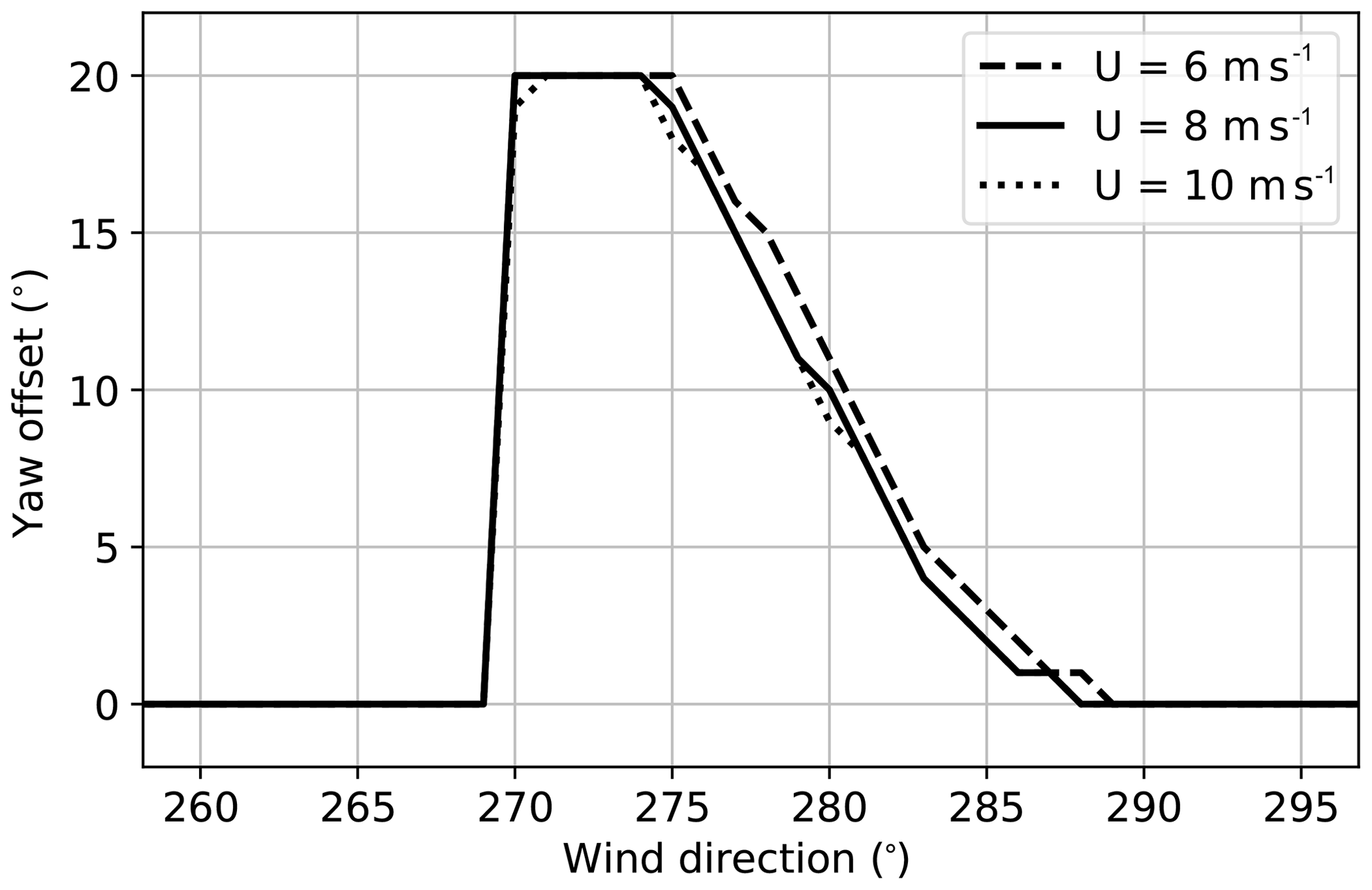
Figure 2Yaw offset schedules optimized for a 5D turbine spacing with static wind directions for mean wind speeds of 6, 8, and 10 m s⁻¹.

Download

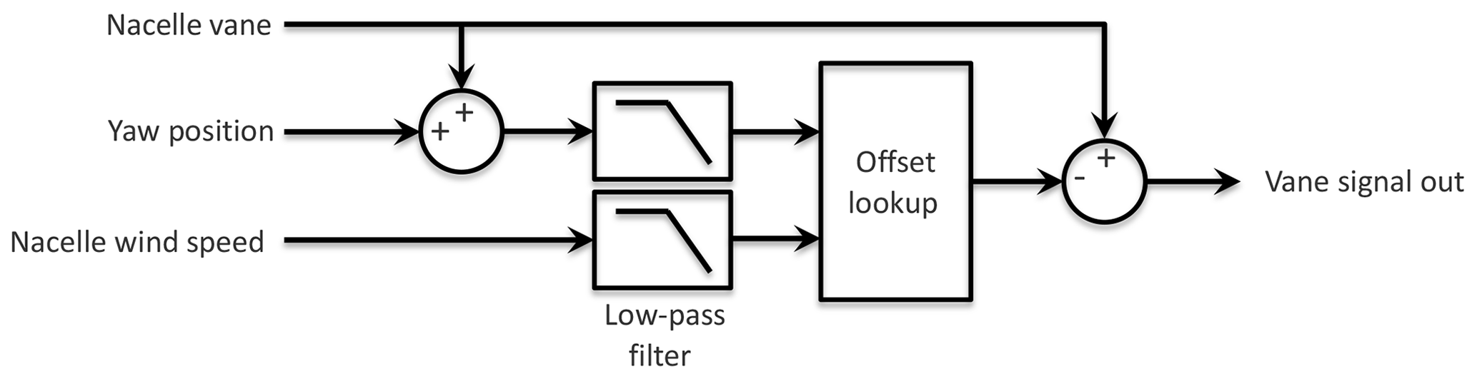
Figure 3Yaw offset controller. Inputs include measurements from the wind turbine's nacelle vane, nacelle anemometer, and yaw position sensor. The output vane signal is used as the input to the wind turbine's yaw controller.

Download

Yaw offset control is used to apply the desired yaw offsets to a turbine and can be implemented as either direct yaw control, wherein a direct yaw position command is sent to the turbine, or indirect yaw control, where the yaw error set point of the standard yaw controller is changed to the target offset. Although more precise yaw offset tracking can be achieved using direct yaw offset control (Bossanyi, 2018), indirect yaw offset control is considered in this research because it can be implemented in the field without modifying the turbine's yaw control logic (Fleming et al., 2019).

The control logic used to implement indirect yaw offset control in this research, which is based on the strategy implemented at a commercial wind farm by Fleming et al. (2019), is provided in Fig. 3. A modified wind vane signal is formed by subtracting the target yaw offset from the original wind vane signal. The modified vane signal is then fed into the wind turbine's standard yaw controller, causing it to track the target yaw offset instead of the default set point of zero. The target yaw offset is determined using a lookup table providing yaw offset as a function of nacelle-based wind speed and direction. Low-pass filtering is applied to the lookup table inputs to provide estimates of the slowly varying mean wind speed and direction. Note that for this study, which considers below-rated operation for U=8 m s⁻¹, the controller is simplified by containing only the yaw offset schedule determined for U=8 m s⁻¹ because of the low sensitivity of the optimal yaw offsets to wind speed variations in this region. After comparing the energy gain resulting from wake steering simulations with different wind direction filter time constants, a value of 30 s was chosen, yielding an estimate of the slowly varying wind direction without introducing too much delay.

2.5 Wind model

To assess wake steering control with wind direction variability, we developed a dynamic wind model representing realistic wind conditions. Time series representing the turbulent wind direction at a point near hub height measured by the nacelle wind vane are needed to simulate the yaw and yaw offset controllers. FLORIS, on the other hand, models the time-averaged wake behavior and power production resulting from turbulent wind conditions as a function of mean wind direction. Additionally, high-frequency, small-scale components of wind direction incorrectly indicate the direction of wake travel. Therefore, a more appropriate input to FLORIS would be a signal representing the slowly varying, large-scale mean wind direction across the wind farm, with the turbulent component removed. To model these two different wind direction signals, stochastic time series are generated representing the slowly varying mean wind direction across the wind farm (the “low-frequency” component) as well as the purely turbulent wind direction component, corresponding to a fixed mean wind direction. The low-frequency component is used as the input to FLORIS, whereas the sum of the two signals acts as the input to the yaw and yaw offset controllers.

As discussed in Sect. 2.4, because wind speed variability around U=8 m s⁻¹ is not expected to significantly impact the effectiveness of wake steering, the wind model is simplified by assuming a fixed free-stream wind speed of 8 m s⁻¹. However, wind speed variability likely has a greater impact on wake steering near rated wind speed, wherein the relationship between wind speed, power, and thrust is more nonlinear.

Stochastic wind direction signals are simulated by generating a normally distributed random time series based on the power spectra of the low-frequency and turbulent wind direction components, assuming the wind directions can be represented as Gaussian random processes. Specifically, a series of Fourier components at discrete frequencies containing uniformly distributed random phases is generated, with magnitudes determined by the desired power spectrum (Shinozuka and Deodatis, 1991). We then apply the inverse discrete Fourier transform to obtain the stochastic time series with a sample period of 1 s.

The power spectrum used to generate the turbulent wind direction component, $S_{{\mathit{\varphi }}_{\mathrm{t}}}\left(f\right)$, is based on data from LES using NREL's SOWFA (Simulator fOr Wind Farm Applications) tool (Churchfield et al., 2012), representing a neutral atmospheric boundary layer with a mean hub height wind speed of $U=\sim \mathrm{8}$ m s⁻¹, which is similar to simulations discussed in past studies (Fleming et al., 2015, 2018). The power spectrum is calculated using data at a height of 95 m with a mean wind speed of U=8.1 m s⁻¹, TI = 10.1 %, and a wind direction standard deviation of 3.93^∘ (see the “LES” spectrum in Fig. 4).

Figure 4Normalized power spectra of the wind direction determined from met mast wind vane measurements, the turbulent wind direction component derived from LES, and the resulting low-frequency wind direction component (a); the same power spectra multiplied by frequency (b).

Download

Measurements obtained from a wind vane at a height of 87 m on the M5 meteorological (met) mast at NREL's National Wind Technology Center (Clifton et al., 2013) are used to determine the power spectrum of the combined low-frequency and turbulent wind directions, S_ϕ(f). To match the conditions generated by LES, data were limited to 1 h periods, wherein the mean wind speed was between 7.5 and 8.5 m s⁻¹ and the atmospheric conditions were neutral (defined using the Monin–Obukhov stability parameter, z∕L; Clifton et al., 2013, at a height of 15 m, as $|z/L|<\mathrm{0.05}$; Rajewski et al., 2013). Using twelve 1 h periods of acceptable data with an average 1 h TI = 18.8 % and an average 1 h wind direction standard deviation of 10.92^∘, a representative wind direction power spectrum is determined, shown as the “Met mast” spectrum in Fig. 4.

Using the power spectra of the LES-based turbulent wind direction component, $S_{{\mathit{\varphi }}_{\mathrm{t}}}\left(f\right)$, and the met-mast-derived combined wind direction, S_ϕ(f), and assuming no correlation between the low-frequency and turbulent components, the spectrum of the low-frequency component, $S_{{\mathit{\varphi }}_{\mathrm{l}}}\left(f\right)$, is found via the relationship

The LES-based turbulent and met-mast-based combined wind direction spectra are compared in Fig. 4, normalized so they converge at high frequencies. Note that the LES-derived spectrum quickly decays above 0.1 Hz because of the spatial filtering inherent in LES. These frequencies are ignored, however, and the trend observed between 0.01 and 0.1 Hz is assumed to continue at higher frequencies. Finally, the wind direction power spectra are approximated using the following equations fit to the data, where $S_{{\mathit{\varphi }}_{\mathrm{l}}}\left(f\right)$ is calculated as $S_{\mathit{\varphi }}\left(f\right)-S_{{\mathit{\varphi }}_{\mathrm{t}}}\left(f\right)$ and C serves as a scaling constant:

Although Eq. (3a) is not physically realistic because it describes a power spectrum containing infinite energy across all frequencies, it fits the data well for the range of frequencies simulated. Note that below 0.0037 Hz, the low-frequency wind direction is the dominant component of the combined wind direction signal; for higher frequencies, the turbulent component dominates. Thus, the low-frequency wind direction component could be estimated by low-pass filtering a measured wind direction time series using a cutoff frequency of 0.0037 Hz.

Examples of the turbulent wind direction and combined wind direction time series from LES and met mast measurements, respectively, are shown in Fig. 5a. Note that the LES is limited to 860 s, whereas the met mast measurements are analyzed in 1 h blocks. Using the power spectra given by Eqs. (3b) and (3c), examples of stochastic time series representing the turbulent and low-frequency wind direction components as well as the combined wind direction, formed by summing the turbulent and low-frequency components, are provided in Fig. 5b. The stochastic time series are scaled to match the combined standard deviation of 10.92^∘ observed in the met mast data.

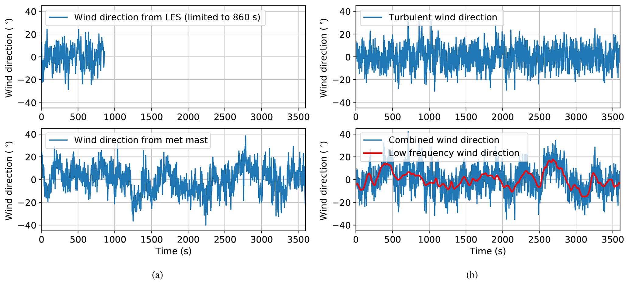
Figure 5Example wind direction time series: (a) wind directions from LES and met mast wind vane measurements and (b) stochastic turbulent, low-frequency, and combined wind directions.

Download

2.6 Simulation procedure

As described in Sect. 2.5, the stochastic low-frequency wind direction component acts as the wind direction used in FLORIS, whereas the combined low-frequency and turbulent wind direction serves as the realistic noisy input to the yaw and yaw offset controllers. A fixed wind speed of 8 m s⁻¹ is used as the input to both FLORIS and the yaw offset controller. Wake steering control is evaluated by generating a series of 1 h stochastic wind direction time series with a combined wind direction standard deviation of 10.92^∘ for a range of mean wind directions. To capture all wind directions wherein wake steering control could be active, unique 1 h simulations are performed for mean wind directions between 200 and 340^∘ in increments of 0.05^∘, resulting in 2800 simulations for each control scenario examined. For comparison purposes, baseline yaw control is simulated in addition to wake steering control for each wind direction time series. The first 10 min of data resulting from each simulation are discarded to eliminate controller start-up transients.

3.1 Wind direction and yaw position uncertainty

Wind direction and yaw position uncertainty are determined by first quantifying the yaw error variability. Standard yaw control is simulated using stochastic low-frequency and combined wind direction signals with the combined wind direction standard deviation of 10.92^∘ measured in the field, as explained in Sect. 2.5. Yaw error variability is then quantified as the standard deviation of the difference between the low-frequency wind direction and the turbine's yaw position. An example of simulated wind direction and yaw position signals for both baseline yaw control and yaw offset control using static-optimal offsets is provided in Fig. 6. Baseline yaw control for the simulated conditions results in a yaw error standard deviation of σ_ϵ=5.25^∘.

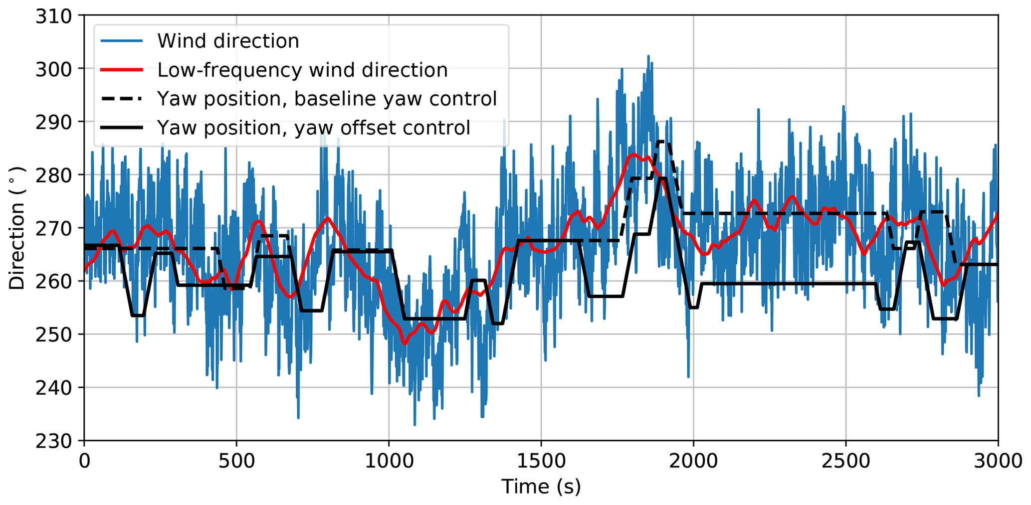
Figure 6Example stochastic wind directions and low-frequency wind directions with yaw positions corresponding to baseline yaw control and yaw offset control, with the 8 m s⁻¹ offset schedule shown in Fig. 2.

Download

The impact of wind direction and yaw position uncertainty on wake steering is analyzed by modeling the low-frequency wind direction (ϕ_l) and yaw position (θ) as jointly distributed random variables formed by adding wind direction and yaw uncertainty to the static wind direction and yaw position defined by the yaw offset schedule. The resulting joint probability density function (PDF) of low-frequency wind direction and yaw position is given by the convolution of the static PDF, $f_{{\mathrm{\Phi }}_{\mathrm{l}},\mathrm{\Theta },\mathrm{s}}({\mathit{\varphi }}_{\mathrm{l}},\mathit{\theta })$, based on the offset schedule, γ(ϕ_l), and the PDF representing the uncertainty in the two variables $f_{{\mathrm{\Delta }}_{\mathrm{\Phi }},{\mathrm{\Delta }}_{\mathrm{\Theta }}}({\mathrm{\Delta }}_{\mathit{\varphi }},{\mathrm{\Delta }}_{\mathit{\theta }})$:

The static PDF of wind direction and yaw position is given by

where δ(⋅) is the Dirac delta function and f_Φ(ϕ) is the PDF of the wind direction, assumed to be uniformly distributed across all wind directions to simplify the analysis. However, f_Φ(ϕ) could easily be replaced by a more appropriate probability distribution based on site-specific conditions.

As explained by Rott et al. (2018), the PDF of the wind direction during a 5 min time period can be approximated as a normal distribution. Because wind turbines typically yaw every few minutes or so – remaining at fixed yaw positions otherwise (see Fig. 6) – the yaw error is also approximated as a normally distributed random variable. The yaw error uncertainty is then divided into wind direction uncertainty, Δ_ϕ, and yaw position uncertainty, Δ_θ, which are treated as independent normally distributed random variables described by the joint PDF:

To maintain the observed yaw error standard deviation of σ_ϵ=5.25^∘, the following relationship between the variances of wind direction uncertainty, yaw position uncertainty, and yaw error must exist:

The impact of the parameters σ_ϕ and σ_θ on the PDF of wind direction and yaw position with wake steering based on the static-optimal offset schedule for 8 m s⁻¹ described in Sect. 2.4 is shown in Fig. 7, which compares theoretical joint PDFs of low-frequency wind direction and yaw position using Eqs. (4) through (7) with a histogram determined from simulation. All theoretical PDFs and histograms are discretized using 1^∘ bins. The theoretical PDF of wind direction and yaw position assuming all of the yaw error variation can be attributed to wind direction uncertainty (σ_ϕ=5.25^∘) is shown in Fig. 7b, whereas the PDF calculated assuming all variation is caused by yaw position uncertainty (σ_θ=5.25^∘) is provided in Fig. 7c. Also shown in the plots are the mean yaw positions achieved as a function of wind direction. Note that the two theoretical PDFs are identical for wind directions far from the yaw offset control sector; for baseline yaw control, any combination of wind direction and yaw position standard deviation that satisfies Eq. (7) produces the same joint PDF of wind direction and yaw position. Consequently, wind directions where wake steering is implemented must be used to identify the proper values of σ_ϕ and σ_θ.

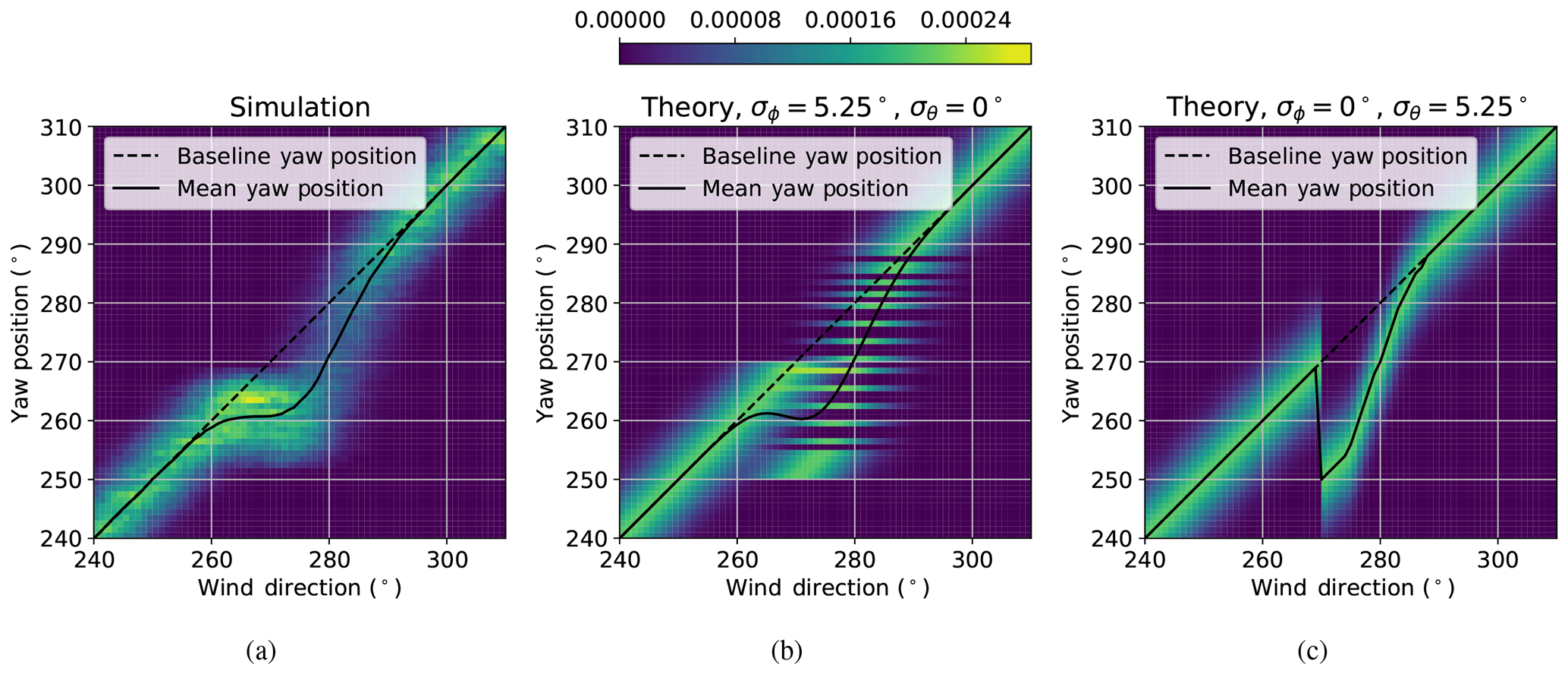
Figure 7Distributions of low-frequency wind direction and yaw position with yaw offset control using a static-optimal yaw offset schedule: (a) histogram from simulation results and theoretical probability density functions assuming (b) only wind direction uncertainty and (c) only yaw position uncertainty.

Download

Rather than attributing all of the yaw error to either yaw position or wind direction uncertainty, Fig. 7 reveals that yaw offset control with wind direction variability is likely modeled best using a combination of the two sources of uncertainty. Assuming all of the yaw error is caused by wind direction uncertainty, as shown in Fig. 7b, implies that the yaw positions determined from the yaw offset schedule are achieved without any uncertainty. But once the yaw offsets are reached, the wind direction varies while the yaw position is fixed, until the turbine yaws again. Note that the yaw position gaps in Fig. 7b are a consequence of discretizing the PDF using 1^∘ bins. Alternatively, Fig. 7c highlights how attributing all of the yaw error to yaw position uncertainty suggests uncertainty in the yaw position that is achieved for a given wind direction but that there is no wind direction variability once the yaw position is reached. The simulation-based histogram in Fig. 7a, however, exhibits characteristics of both yaw position and wind direction uncertainty. Because the mean yaw positions achieved based on the simulation results are closer to the theoretical mean yaw values with no yaw position uncertainty, most of the yaw error can likely be attributed to wind direction uncertainty, as modeled by Rott et al. (2018). The procedure used to quantify the amount of wind direction and yaw position uncertainty, described by σ_ϕ and σ_θ, respectively, used in the remainder of this research is explained in Sect. 3.3.

3.2 Yaw offset optimization procedure

For a given estimated low-frequency wind direction, ${\widehat{\mathit{\varphi }}}_{\mathrm{l}}$, determined by the yaw offset controller, the optimal yaw offset γ^* for the upstream turbine in the turbine pair is found using

where $E\left[P\right({\widehat{\mathit{\varphi }}}_{\mathrm{l}},\mathit{\gamma }\left)\right]$ is the expected power production given the estimated wind direction, ${\widehat{\mathit{\varphi }}}_{\mathrm{l}}$, and target yaw offset, γ. Based on the joint probability distribution of wind direction and yaw position uncertainty in Eq. (6), the expected power production using FLORIS is given by

where P_FLORIS(ϕ_l,γ) describes the power production of the two-turbine array as a function of low-frequency wind direction and the yaw offset of the upstream turbine, and Δ_ϕ and Δ_θ represent deviations of the wind direction and yaw position from their mean values, respectively. Equations (8) and (9) essentially comprise the same form of optimization used by Quick et al. (2017), considering only yaw uncertainty, and Rott et al. (2018), examining wind direction uncertainty. Equation (9) is implemented by approximating the integration as a double summation and discretizing wind direction and yaw position using a step size of 1^∘. As a result, only integer yaw offset values are considered.

The solution to Eqs. (8) and (9) as a function of wind direction without wind direction or yaw position uncertainty (${\mathit{\sigma }}_{\mathit{\varphi }}={\mathit{\sigma }}_{\mathit{\theta }}=\mathrm{0}$) yields the static-optimal yaw offset schedule. When wind direction and yaw uncertainty, resulting from wind direction variability, are included, the solution is referred to as the dynamic-optimal offset schedule.

3.3 Wind direction and yaw position variability parameter tuning

Appropriate values for the standard deviation of the wind direction and yaw uncertainty are found by comparing the expected mean energy production with wake steering based on theoretical PDFs of wind direction and yaw with simulation results. Specifically, the mean energy production across all wind directions is calculated for different combinations of σ_ϕ and σ_θ adhering to Eq. (7). The combination that best predicts the mean energy resulting from wake steering simulations is used for finding the dynamic-optimal yaw offset schedule. Note that we assume the controller has perfect knowledge of the yaw position. Yaw uncertainty, as defined here, instead stems from the dynamics and hysteresis of the yaw and wake steering controllers. For example, the target yaw misalignment determined by the yaw offset controller lags behind the true wind direction, which can cause the yaw controller to settle on an unintended yaw position. Additionally, while the turbine is yawing to achieve a particular yaw misalignment, the offset target from the yaw offset controller can change, again causing the controller to stop at an unintended yaw position.

To find the uncertainty parameters that best predict the energy production with dynamic-optimal yaw offsets, an iterative parameter tuning approach is used. An initial guess is made, setting yaw position uncertainty equal to wind direction uncertainty. Next, simulation results based on the initial dynamic-optimal yaw offset schedule are used to retune the uncertainty parameters. The process is repeated until both the uncertainty parameters and optimal yaw offsets converge. By applying this tuning procedure, values of σ_ϕ=4.95 and σ_θ=1.75^∘ are found. As expected, most of the yaw error variation is attributed to wind direction uncertainty, with a small amount of yaw position uncertainty caused by the yaw controller dynamics. A comparison between the histogram of low-frequency wind direction and yaw position based on wake steering simulations using the dynamic-optimal yaw offset schedule and the theoretical joint PDF with σ_ϕ=4.95 and σ_θ=1.75^∘ is shown in Fig. 8.

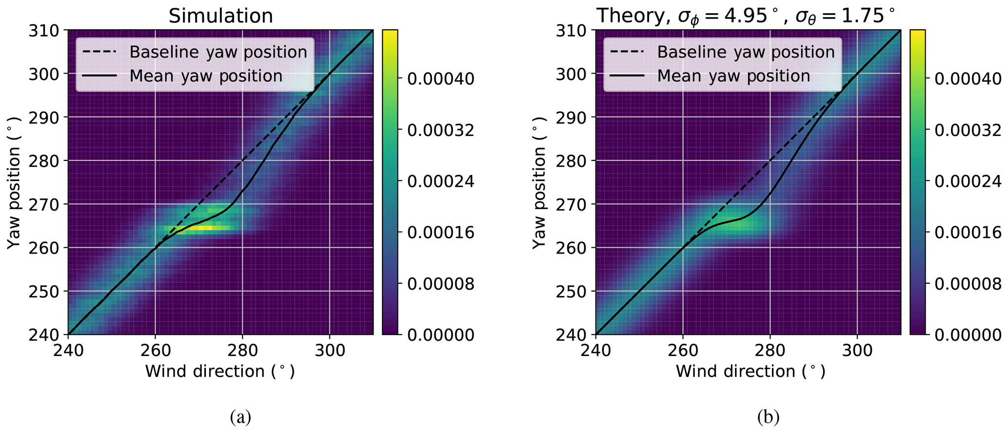
Figure 8Distributions of low-frequency wind direction and yaw position with yaw offset control using a dynamic-optimal yaw offset schedule: (a) histogram from simulation results and (b) theoretical probability density function assuming wind direction uncertainty with a standard deviation of 4.95^∘ and yaw position uncertainty with a standard deviation of 1.75^∘.

Download

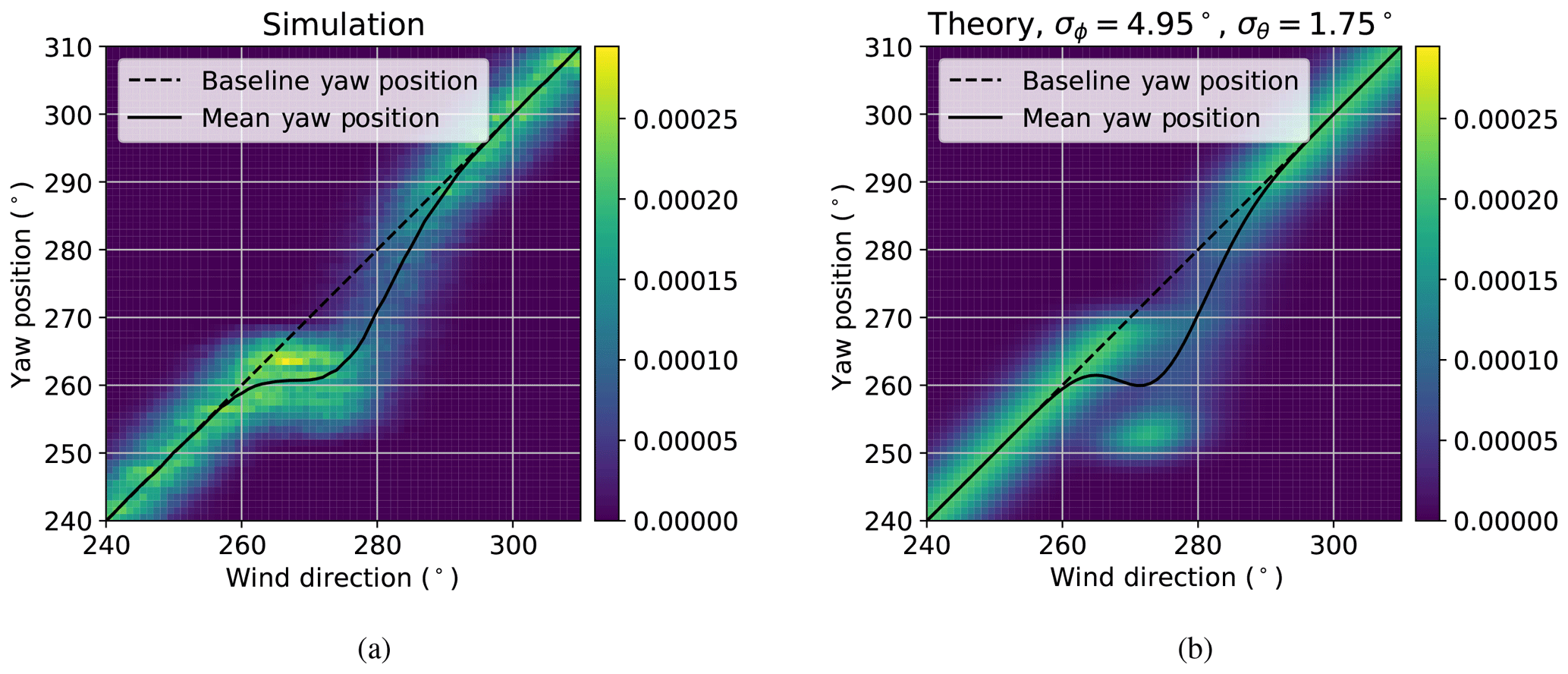
Figure 9Distributions of low-frequency wind direction and yaw position with yaw offset control using a static-optimal yaw offset schedule: (a) histogram from simulation results and (b) theoretical probability density function assuming wind direction uncertainty with a standard deviation of 4.95^∘ and yaw position uncertainty with a standard deviation of 1.75^∘.

Download

A comparison between the histogram of low-frequency wind direction and yaw position from wake steering simulations with the original static-optimal yaw offset schedule from Fig. 2 and the theoretical joint PDF using the tuned parameters is shown in Fig. 9. Although the mean yaw positions are similar, the wind direction and yaw distributions do not match as well as they do for the dynamic-optimal case, especially near ϕ=270^∘, where the wind direction is aligned with the turbine pair. Close agreement is desired so that the theoretical joint PDF of wind direction and yaw position can be used to accurately predict the simulated energy gain, allowing the optimal yaw offset schedule to be reliably found using the theoretical PDF. Part of this discrepancy can be explained by the larger offsets demanded by the static-optimal offset schedule. The theoretical joint PDF of wind direction and yaw assumes that the yaw controller tends to settle near one of the two yaw position extremes near ϕ=270^∘. However, the wake steering simulations reveal that the yaw controller often settles between the two extremes in this region as a result of the indirect yaw control implementation. Thus, the specific yaw control dynamics affect how well the theoretical joint PDF of wind direction and yaw predicts the actual control behavior. Notwithstanding the observed discrepancies for the static-optimal offset schedule, there is good agreement between the simulated and predicted joint PDFs for the robust dynamic-optimal case.

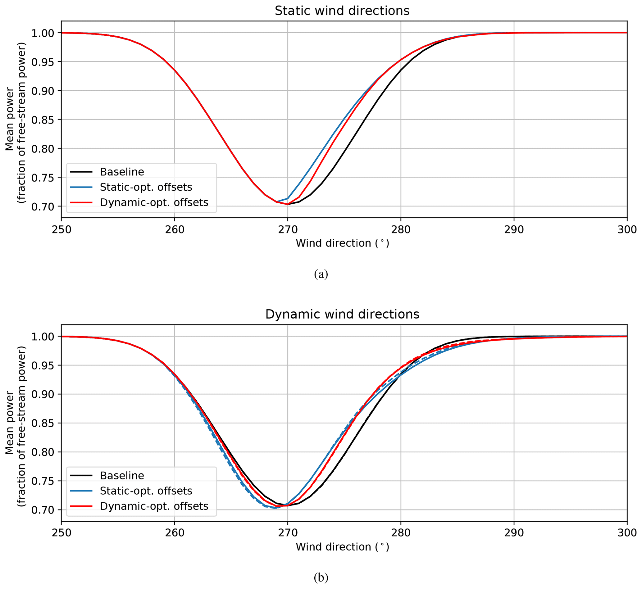
Figure 10Normalized mean power of combined upstream and downstream turbines for baseline and wake steering control with static-optimal and dynamic-optimal yaw offset schedules for (a) static and (b) dynamic wind directions. Mean power values are determined from theory (solid) and simulation (dashed) for a turbine spacing of 5D and turbulence intensity of 10 % and plotted as a function of low-frequency wind direction.

Download

4.1 Comparison of yaw offset controllers optimized for static and variable wind directions

For a turbine spacing of 5D and turbulence intensity of 10 %, the normalized mean power of the combined upstream and downstream turbines binned by low-frequency wind direction for westerly wind directions is shown in Fig. 10 for baseline yaw control and wake steering control. The mean power production resulting from baseline yaw control and wake steering control with static-optimal and dynamic-optimal yaw offsets is provided in Fig. 10a for the case of static wind directions (i.e., power is computed for each wind direction independently, with yaw offsets determined directly from the yaw offset schedules). Clearly, the static-optimal offset schedule outperforms the lower-magnitude dynamic-optimal yaw offsets in this case. Note that power is only increased for one-half of the waked sector because of the restriction of positive yaw offsets. Figure 10b shows the mean power produced with the same three control scenarios with wind direction variability included. Solid lines correspond to theoretical predictions of power production based on Eq. (9), whereas dashed lines are calculated from simulation results. Here, the static-optimal yaw offsets only outperform the dynamic-optimal offsets in a narrow sector; overall, the dynamic-optimal yaw offsets result in higher energy gain. Because of wind direction variability, the applied yaw offsets cause a loss in power when the wind direction drops below 270^∘ or increases above ∼280^∘. Compared to the static-optimal offsets, the dynamic-optimal yaw offset schedule strikes a balance between achieving large gains between 270 and ∼280^∘ and minimizing losses outside this sector.

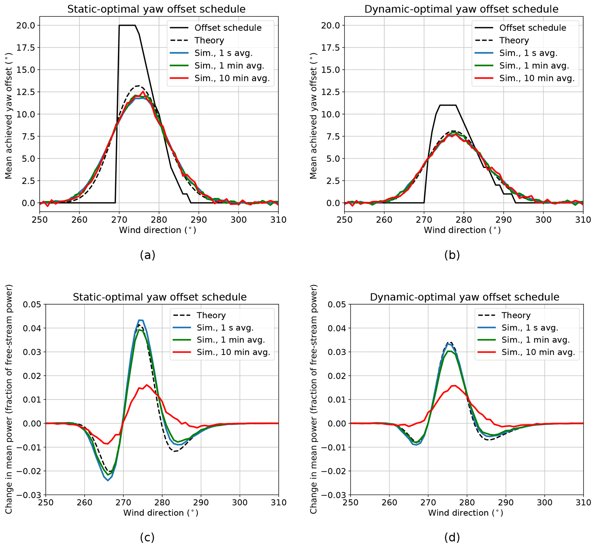
Figure 11Mean achieved yaw offsets using offset schedules optimized for (a) static and (b) dynamic wind directions as well as change in mean power produced by the turbine pair from wake steering using offset schedules optimized for (c) static and (d) dynamic wind directions as a function of low-frequency wind direction. Theoretical achieved offsets and power gains are shown for dynamic wind directions along with the yaw offset schedules. Achieved yaw offsets and power gains from simulations with dynamic wind directions are provided for 1 s, 1 min, and 10 min averages of low-frequency wind direction, yaw offset, and power. A turbine spacing of 5D and turbulence intensity of 10 % are used in the FLORIS model.

Download

Mean yaw offsets along with the normalized change in power produced by the turbine pair with wake steering control are plotted in Fig. 11 as a function of low-frequency wind direction for both static-optimal and dynamic-optimal yaw offsets. The mean achieved yaw offsets and changes in power with dynamic wind directions predicted by theory and resulting from simulation are shown along with the yaw offset schedules. Simulation results are provided based on binning using the original 1 s data as well as 1 and 10 min averages of the data. The mean achieved yaw offsets binned by low-frequency wind direction for the static-optimal and dynamic-optimal cases reveal the source of the power loss below 270 and above ∼280^∘, as shown in Fig. 10b. For wind directions below 270^∘, zero yaw offset is desired. However, the positive mean yaw offsets resulting from wind direction variability cause the wake to deflect clockwise toward the downstream turbine, reducing its power. On the other hand, for wind directions above ∼280^∘, relatively small yaw offsets are needed to deflect the partial wake away from the downstream turbine. Because of wind direction variability, the resulting mean yaw offsets are too large, leading to unnecessary power loss on the upstream turbine with little additional gain at the downstream turbine. Comparing the static-optimal and dynamic-optimal cases shows how the less-aggressive dynamic-optimal yaw offsets lead to slightly lower peak gains in power production, but they result in lower mean yaw offsets achieved outside of the primary wake steering region, minimizing power loss. The lower peak gains are more than compensated for by the reduced losses. Finally, note that the dynamic-optimal yaw offsets extend to higher wind directions than the static-optimal offsets. The small offsets above 290^∘ result in very little power loss, yet, due to wind direction variability, help increase the mean achieved yaw offsets at lower wind directions where wake steering is beneficial.

Table 1Percentage of wake losses recovered from wake steering with dynamic wind directions for a two-turbine array with different turbine spacings and turbulence intensity values, assuming uniformly distributed wind directions. Results are provided for static-optimal and dynamic-optimal yaw offsets based on theoretical predictions as well as simulations.

Download Print Version | Download XLSX

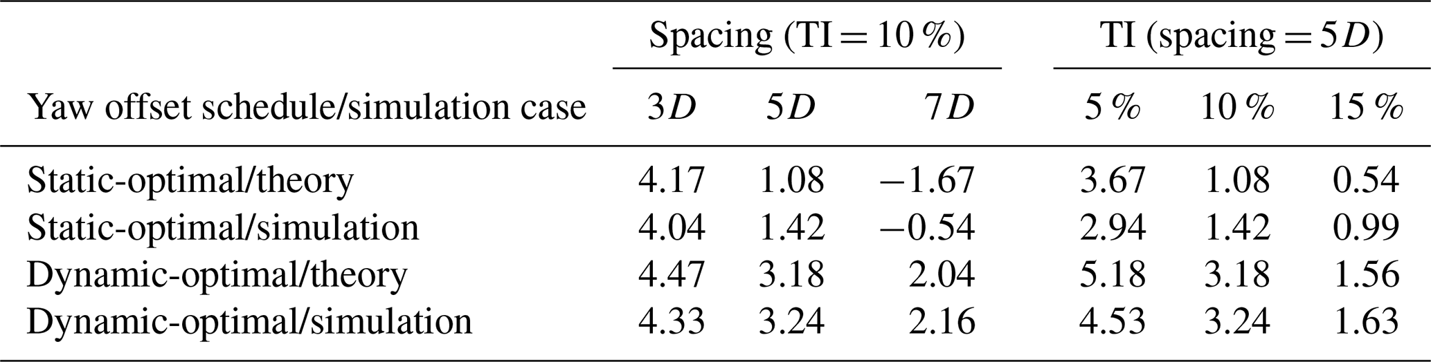
Table 2Total baseline wake losses compared to free-stream operation for a two-turbine array with different turbine spacings and turbulence intensity values, assuming uniformly distributed wind directions.

Download Print Version | Download XLSX

The theoretical predictions of the mean achieved yaw offsets and change in power with wake steering match the simulation results very well for the dynamic-optimal yaw offset scenario in Fig. 11b and d, for which the wind direction and yaw position uncertainty model is tuned. For the static-optimal scenario, the theory predicts higher peak mean yaw offsets and a more narrow achieved yaw offset region than exhibited by the simulations. The predicted change in power also differs from the simulations more than in the dynamic-optimal case. As explained in Sect. 3.3, these discrepancies are related to yaw controller dynamics that are unaccounted for in the theoretical predictions.

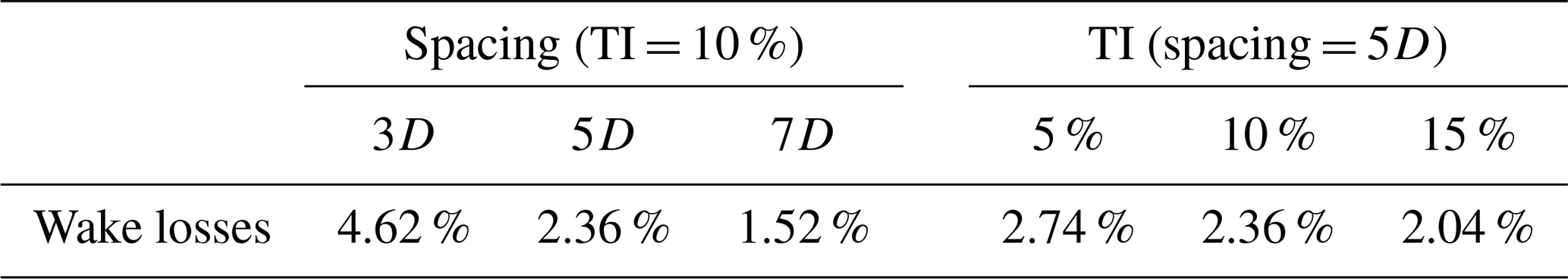
The overall gains for different wake steering scenarios are provided in Table 1, which lists the percentage of the total wake losses recovered with dynamic wind directions assuming uniformly distributed wind directions. The baseline wake losses for the different scenarios investigated, from which the wake loss recovery is calculated, are provided in Table 2, again assuming uniformly distributed wind directions. Note that when averaging over all wind directions, the gain in absolute energy production from wake steering is small for this two-turbine scenario (≤0.2 %), primarily because of the low baseline wake losses. Therefore, we express the gains as a percentage of wake losses recovered, which we expect to be a more meaningful value for comparison across different wind farm scenarios. When simulating dynamic wind directions, 1.42 % of the wake losses are recovered by the static-optimal offset schedule. The theoretical prediction of 1.08 % slightly underestimates the energy gain because of unmodeled yaw controller dynamics, indicating room for improvement in the theoretical model. By accounting for wind direction and yaw position uncertainty, wake steering simulations using dynamic-optimal yaw offsets result in an energy gain of 3.24 % of total wake losses, nearly matching the predicted increase of 3.18 % and representing more than a 2-fold improvement over the static-optimal wake steering case.

Simulation results in Fig. 11 are binned using different averaging periods to illustrate how longer averaging periods can hide or smooth out some of the trends predicted by the theory. Averaging periods of 1 or 10 min are more relevant when analyzing field data because of uncertainty in high-frequency wind direction measurements and to account for the time it takes for the wake to propagate between the pair of turbines. Although the mean achieved yaw offsets are not sensitive to these averaging periods, the mean change in power shows a strong dependence on the averaging period used for binning. As the binning period increases, the mean power trends are smoothed out. For example, using 10 min averages, the simulation results for the dynamic-optimal scenario almost completely hide the power loss outside the main wake steering region and show a lower peak gain instead.

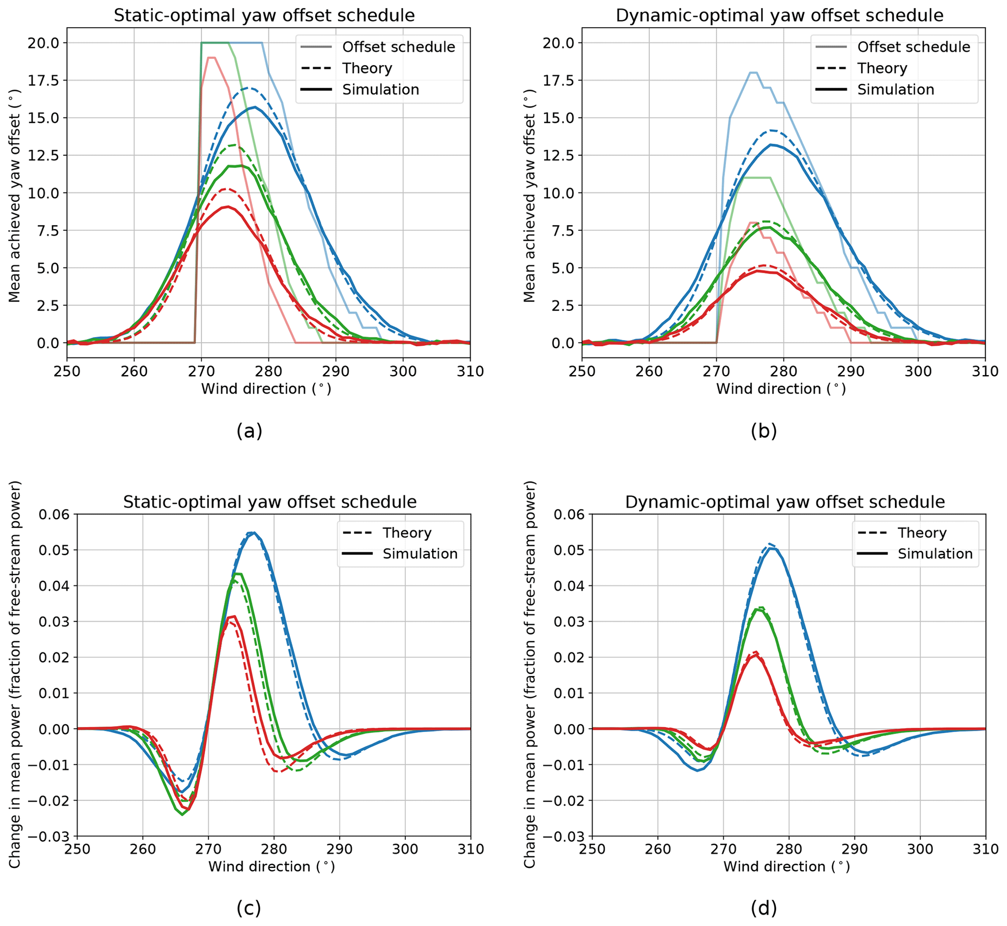
Figure 12Mean achieved yaw offsets using offset schedules optimized for (a) static and (b) dynamic wind directions as well as change in mean power produced by the turbine pair from wake steering using offset schedules optimized for (c) static and (d) dynamic wind directions as a function of low-frequency wind direction for turbine spacings of 3D (blue), 5D (green), and 7D (red). Achieved theoretical and simulation-based offsets and power gains are shown for dynamic wind directions, along with the yaw offset schedules. A turbulence intensity of 10 % is used in the FLORIS model.

Download

4.2 Impact of turbine spacing

For a two-turbine array, the turbine spacing impacts both the amount of energy that can be gained using wake steering and the additional benefit from using a dynamic-optimal yaw offset strategy. Keeping all other wind farm parameters the same as in Sect. 4.1, Fig. 12 compares the mean yaw offsets and change in power produced by the turbine pair as a function of low-frequency wind direction for both static-optimal and dynamic-optimal offset schedules for turbine spacings of 3, 5, and 7D, based on theory and simulation. Figure 12 shows that more energy can be gained using wake steering for shorter separation distances, where wake losses are higher (see Table 2). As the separation distance increases, baseline wake losses become lower, leaving less room for wake steering to improve energy production. However, as the separation distance increases, the wake steering losses suffered because of wind direction variability increase. As shown by the simulation results in Table 1, for a spacing of 3D, wake steering control in dynamic wind conditions using the static-optimal offset schedule results in a wake loss recovery of 4.04 %, whereas with the 7D spacing, energy is reduced compared to the baseline case, yielding a wake loss recovery of −0.54 %. Longer separation distances allow more time for a redirected wake to deflect by the time it reaches the downstream turbine. Consequently, unintended deviations from the optimal yaw offset result in larger changes to the wake position at the downstream turbine. For example, note the relatively high losses below 270^∘ for the 7D spacing with static-optimal yaw offsets in Fig. 12c caused by mean positive yaw offset angles, which significantly redirect the wake toward the downstream turbine.

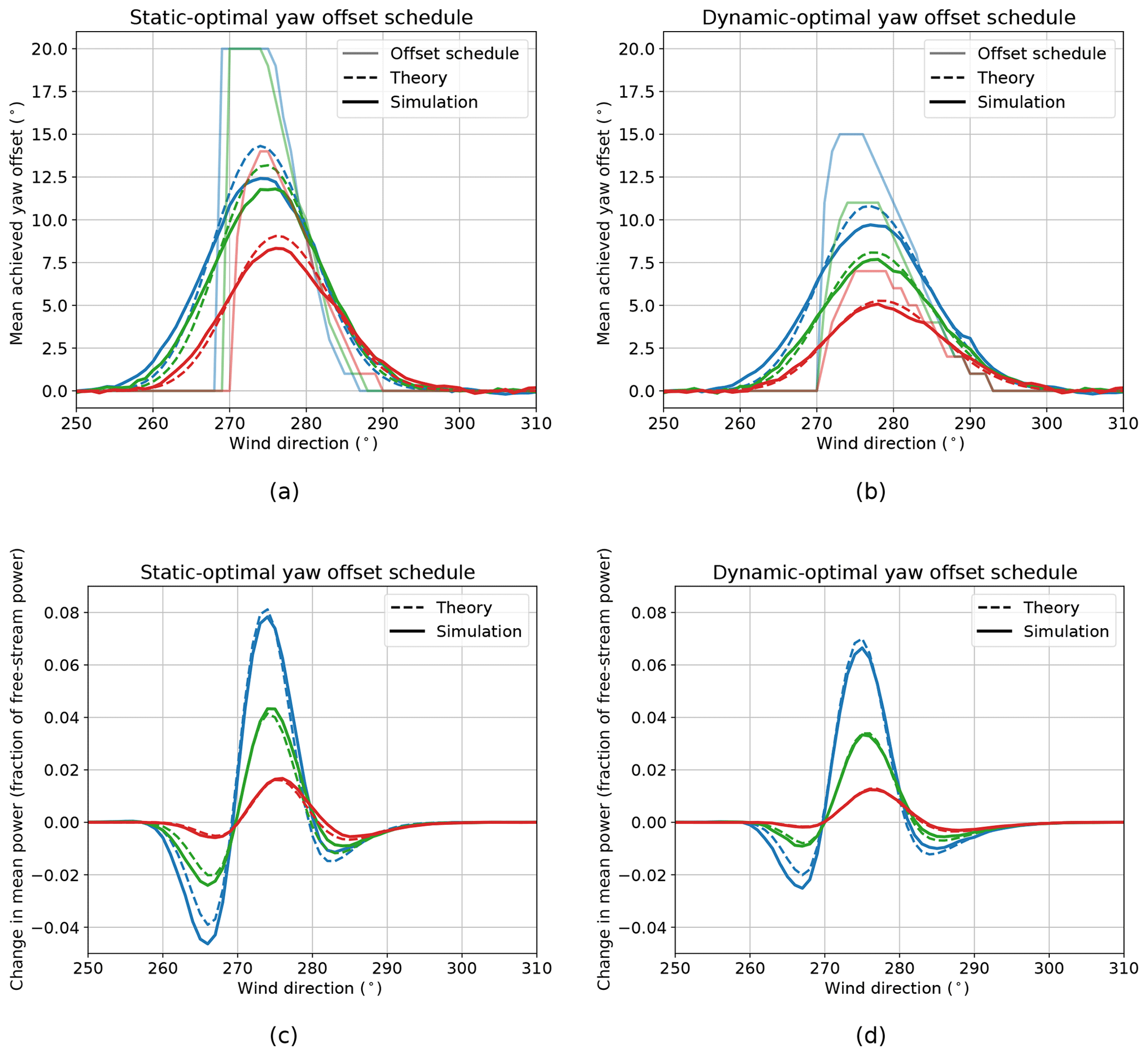
Figure 13Mean achieved yaw offsets using offset schedules optimized for (a) static and (b) dynamic wind directions as well as change in mean power produced by the turbine pair from wake steering using offset schedules optimized for (c) static and (d) dynamic wind directions as a function of low-frequency wind direction for turbulence intensity values of 5 % (blue), 10 % (green), and 15 % (red). Achieved theoretical and simulation-based offsets and power gains are shown for dynamic wind directions, along with the yaw offset schedules. A turbine spacing of 5D is used in the FLORIS model.

Download

Because the reduction in energy gain from wake steering caused by wind direction variability increases for larger turbine separations, the relative importance of using dynamic-optimal offset schedules increases as well. As shown in Fig. 12b and d, to achieve robustness for wind direction and yaw uncertainty, the peak dynamic-optimal offsets become smaller as the separation distance and, therefore, sensitivity to yaw offset deviations become greater. As a result, although the peak power gains are lower than with static-optimal yaw offsets, the losses below 270^∘ and above the primary wake steering sector are greatly reduced. Referring to Table 1, for a separation of 3D, replacing the static-optimal offsets with the dynamic-optimal offset schedule only raises the energy gained by wake steering from 4.04 % of the total wake losses to 4.33 %. But for a spacing of 7D, switching to dynamic-optimal offsets changes the energy loss resulting from static-optimal offsets to an energy gain of 2.16 % of total wake losses.

4.3 Impact of turbulence intensity

Just as wake steering can be implemented for a variety of turbine spacings, the effectiveness of wake steering depends on the atmospheric conditions. Although atmospheric stability has been shown to have a large impact on wake steering (Vollmer et al., 2016; Fleming et al., 2019), ambient turbulence intensity (TI), which is closely linked to stability, acts as the primary atmospheric variable in the Gaussian wake model used in this research (Niayifar and Porté-Agel, 2016), affecting the degree of wake expansion and recovery. Turbulence causes the low-velocity air in the wake to mix with the surrounding higher-velocity flow, helping the wake recover. Additionally, turbulence causes wake meandering. Therefore, low TI leads to a narrow time-averaged wake profile with a high peak wake loss, whereas high turbulence causes a broader wake profile with lower peak losses. As listed in Table 2, the total wake losses decrease as the TI increases.

For a fixed turbine spacing of 5D, Fig. 13 shows the offset schedules, mean achieved yaw offsets, and changes in power of the turbine pair resulting from wake steering as a function of low-frequency wind direction using both static-optimal and dynamic-optimal offsets for TI values of 5 %, 10 %, and 15 %. The low-turbulence case with TI = 5 % allows the greatest amount of energy to be gained using wake steering; with a narrow wake profile with deep losses, wake deflection causes a larger increase in velocity at the downstream turbine than for a more spread-out wake profile with lower velocity deficits typical of high turbulence. At the same time, the higher sensitivity of the power production to changes in yaw offset also means that unintended yaw offsets can more easily steer the wake center back toward the downstream turbine, reducing power, as shown in Fig. 13c, between 260 and 270^∘. Because the greater susceptibility to wind direction and yaw position uncertainty outside of the primary wake steering control sector for lower TI values is somewhat balanced by the higher peak power gains inside the control sector, the relative impact of wind direction variability on the effectiveness of wake steering remains roughly constant as TI varies.

Similar to the results in Fig. 12, while the peak energy gains with dynamic-optimal offsets shown in Fig. 13d are lower than they are with static-optimal offset schedules, because of more robust, lower-magnitude offsets shown in Fig. 13b, the energy lost outside of the primary wake steering sector is greatly reduced. But just as the impact of wind direction variability on the overall effectiveness of wake steering does not strongly depend on TI, the relative improvement in the energy gain made possible by replacing static-optimal offset schedules with dynamic-optimal yaw offsets does not exhibit a clear trend with TI. The largest relative improvement in energy production after switching to dynamic-optimal yaw offsets occurs for the middle TI value of 10 %, where the percentage of wake losses recovered by wake steering increases from 1.42 % to 3.24 % (a relative improvement of 128 %). However, large improvements in energy gains from wake steering are observed for both the lower and higher TI values as well (see Table 1). For TI = 5 %, the energy gain increases from 2.94 % of total wake losses to 4.53 % when dynamic-optimal offsets are used (a relative change of 54 %). Similarly, after switching to the dynamic-optimal yaw offset schedule, the wake loss recovery for TI = 15 % increases from 0.99 % to 1.63 % (a relative change of 65 %).